Center manifold

In the mathematics of evolving systems, the concept of a center manifold was originally developed to determine stability of degenerate equilibria. Subsequently, the concept of center manifolds was realised to be fundamental to mathematical modelling.

Center manifolds play an important role in bifurcation theory because interesting behavior takes place on the center manifold and in multiscale mathematics because the long time dynamics of the micro-scale often are attracted to a relatively simple center manifold involving the coarse scale variables.

Informal example

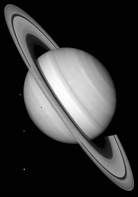
Saturn's rings sit in the center manifold defined by tidal forces.

Saturn's rings provide a rough example of the center manifold of the tidal forces acting on particles within the rings. Tidal forces have a characteristic "compress and stretch" action on bodies, with the compressing direction defining the stable manifold, the stretching direction defining the unstable manifold, and the neutral direction being the center manifold. In the case of Saturn, a particle in orbit above or below the rings will cross the rings, and, from the viewpoint of the rings, it will appear to oscillate from above to below the plane and back. Thus, it appears that the rings are "attractive". Friction, via collisions with other particles in the rings, will dampen those oscillations; thus they will decrease. Such converging trajectories are characteristic of the stable manifold: particles in the stable manifold come closer together. Particles within the ring will have an orbital radius that is a random walk: as they meet in close encounters with other particles in the ring, they will exchange energy in those encounters, and thus alter their radius. In this sense, the space where the rings lie is neutral: there are no further forces upwards or downwards (out of the plane of the rings), nor inwards or outwards (changing the radius within the rings).

This example is a bit confusing, as, properly speaking, the stable, unstable and neutral manifolds do not divide up the coordinate space; they divide up the phase space. In this case, the phase space has the structure of a tangent manifold: for every point in space (a 3D position), there is the collection of "tangent vectors": all possible velocities a particle might have. Some position-velocity pairs are driven towards the center manifold, others are flung away from it. Those that are in the center manifold are susceptible to small perturbations that generally push them about randomly, and often push them out of the center manifold. That is, small perturbations tend to destabilize points in the center manifold: the center manifold behaves like a saddle point, or rather, an extended collection of saddle points. There are dramatic counterexamples to this idea of instability at the center manifold; see Lagrangian coherent structure for detailed examples.

A much more sophisticated example is the Anosov flow on tangent bundles of Riemann surfaces. In that case, one can write a very explicit and precise splitting of the tangent space into three parts: the unstable and stable bundles, with the neutral manifold wedged in the middle between these two. This example is elegant, in the sense that it does not require any approximations or hand-waving: it is exactly solvable. It is a relatively straightforward and simple example for those acquainted with the general outline of Lie groups and Riemann surfaces.

Definition

Center (red) and unstable (green) manifolds of saddle-node equilibrium point of the system

{\dot {x}}=x^{2},

{\dot {y}}=y

.

Randomly selected points of the 2D phase space converge exponentially to a 1D center manifold on which dynamics are slow (non exponential). Studying dynamics of the center manifold determines the stability of the non-hyperbolic fixed point at the origin.

The center manifold of a dynamical system is based upon an equilibrium point of that system. A center manifold of the equilibrium then consists of those nearby orbits that neither decay exponentially quickly, nor grow exponentially quickly.

Mathematically, the first step when studying equilibrium points of dynamical systems is to linearize the system, and then compute its eigenvalues and eigenvectors. The eigenvectors (and generalized eigenvectors if they occur) corresponding to eigenvalues with negative real part form a basis for the stable eigenspace. The (generalized) eigenvectors corresponding to eigenvalues with positive real part form the unstable eigenspace. If the equilibrium point is hyperbolic (that is, all eigenvalues of the linearization have nonzero real part), then the Hartman-Grobman theorem guarantees that these eigenvalues and eigenvectors completely characterise the systems dynamics near the equilibrium.

However, if the equilibrium has eigenvalues whose real part is zero, then the corresponding (generalized) eigenvectors form the center eigenspace—for a ball, the center eigenspace is the entire set of unforced rigid body dynamics. [1] Going beyond the linearization, when we account for perturbations by nonlinearity or forcing in the dynamical system, the center eigenspace deforms to the nearby center manifold. [2] If the eigenvalues are precisely zero (as they are for the ball), rather than just real-part being zero, then the corresponding eigenspace more specifically gives rise to a slow manifold. The behavior on the center (slow) manifold is generally not determined by the linearization and thus may be difficult to construct.

Analogously, nonlinearity or forcing in the system perturbs the stable and unstable eigenspaces to a nearby stable manifold and nearby unstable manifold.[3] These three types of manifolds are three cases of an invariant manifold.

Algebraically, let ${\frac {d{\textbf {x}}}{dt}}={\textbf {f}}({\textbf {x}})$ be a dynamical system with equilibrium point ${\textbf {x}}^{*}$ . The linearization of the system near the equilibrium point is

{\frac {d{\textbf {x}}}{dt}}=A{\textbf {x}},\quad {\text{where }}A={\frac {d{\textbf {f}}}{d{\textbf {x}}}}({\textbf {x}}^{*}).

The Jacobian matrix $A$ defines three main subspaces:

the stable subspace, which is spanned by the generalized eigenvectors corresponding to the eigenvalues $\lambda$ with $\operatorname {Re} \lambda <0$ ;
the unstable subspace, which is spanned by the generalized eigenvectors corresponding to the eigenvalues $\lambda$ with $\operatorname {Re} \lambda >0$ ;
the center subspace, which is spanned by the generalized eigenvectors corresponding to the eigenvalues $\lambda$ with $\operatorname {Re} \lambda =0$ .

Depending upon the application, other subspaces of interest include center-stable, center-unstable, sub-center, slow, and fast subspaces. These subspaces are all invariant subspaces of the linearized equation.

Corresponding to the linearized system, the nonlinear system has invariant manifolds, each consisting of sets of orbits of the nonlinear system.[4]

An invariant manifold tangent to the stable subspace and with the same dimension is the stable manifold.
The unstable manifold is of the same dimension and tangent to the unstable subspace.
A center manifold is of the same dimension and tangent to the center subspace. If, as is common, the eigenvalues of the center subspace are all precisely zero, rather than just real part zero, then a center manifold is often called a slow manifold.

Center manifold theorems

The center manifold existence theorem states that if the right-hand side function ${\textbf {f}}({\textbf {x}})$ is $C^{r}$ ( $r$ times continuously differentiable), then at every equilibrium point there exists a neighborhood of some finite size in which there is at least one of [5]

a unique $C^{r}$ stable manifold,
a unique $C^{r}$ unstable manifold,
and a (not necessarily unique) $C^{r-1}$ center manifold.

In example applications, a nonlinear coordinate transform to a normal form can clearly separate these three manifolds.[6] A web service currently undertakes the necessary computer algebra for a range of finite-dimensional systems.

In the case when the unstable manifold does not exist, center manifolds are often relevant to modelling. The center manifold emergence theorem then says that the neighborhood may be chosen so that all solutions of the system staying in the neighborhood tend exponentially quickly to some solution ${\textbf {y}}(t)$ on the center manifold. That is, ${\textbf {x}}(t)={\textbf {y}}(t)+{\mathcal {O}}(e^{-\beta 't})\quad {\text{as }}t\to \infty \,,$ for some rate $\beta '$ . [7] This theorem asserts that for a wide variety of initial conditions the solutions of the full system decay exponentially quickly to a solution on the relatively low dimensional center manifold.

A third theorem, the approximation theorem, asserts that if an approximate expression for such invariant manifolds, say ${\textbf {x}}={\textbf {X}}({\textbf {s}})$ , satisfies the differential equation for the system to residuals ${\mathcal {O}}(|{\textbf {s}}|^{p})$ as ${\textbf {s}}\to {\textbf {0}}$ , then the invariant manifold is approximated by ${\textbf {x}}={\textbf {X}}({\textbf {s}})$ to an error of the same order, namely ${\mathcal {O}}(|{\textbf {s}}|^{p})$ .

Center manifolds of infinite-D and/or of non-autonomous systems

However, some applications, such as to dispersion in tubes or channels, require an infinite-dimensional center manifold. [8] The most general and powerful theory was developed by Aulbach and Wanner. [9] [10] [11] They addressed non-autonomous dynamical systems ${\frac {d{\textbf {x}}}{dt}}={\textbf {f}}({\textbf {x}},t)$ in infinite dimensions, with potentially infinite dimensional stable, unstable and center manifolds. Further, they usefully generalised the definition of the manifolds so that the center manifold is associated with eigenvalues such that $|\operatorname {Re} \lambda |\leq \alpha$ , the stable manifold with eigenvalues $\operatorname {Re} \lambda \leq -\beta <-r\alpha$ , and unstable manifold with eigenvalues $\operatorname {Re} \lambda \geq \beta >r\alpha$ . They proved existence of these manifolds, and the emergence of a center manifold, via nonlinear coordinate transforms.

Potzsche and Rasmussen established a corresponding approximation theorem for such infinite dimensional, non-autonomous systems. [12]

Alternative backwards theory

All the extant theory mentioned above seeks to establish invariant manifold properties of a specific given problem. In particular, one constructs a manifold that approximates an invariant manifold of the given system. An alternative approach is to construct exact invariant manifolds for a system that approximates the given system---called a backwards theory. The aim is to usefully apply theory to a wider range of systems, and to estimate errors and sizes of domain of validity. [13] [14]

This approach is cognate to the well-established backward error analysis in numerical modeling.

Center manifold and the analysis of nonlinear systems

As the stability of the equilibrium correlates with the "stability" of its manifolds, the existence of a center manifold brings up the question about the dynamics on the center manifold. This is analyzed by the center manifold reduction, which, in combination with some system parameter μ, leads to the concepts of bifurcations.

Correspondingly, two web services currently undertake the necessary computer algebra to construct just the center manifold for a wide range of finite-dimensional systems (provided they are in multinomial form).

One web service constructs slow manifolds for systems which are linearly diagonalised, but which may be non-autonomous or stochastic.[15]
Another web service constructs center manifolds for systems with general linearisation, but only for autonomous systems.[16]

Examples

The Wikipedia entry on slow manifolds gives more examples.

A simple example

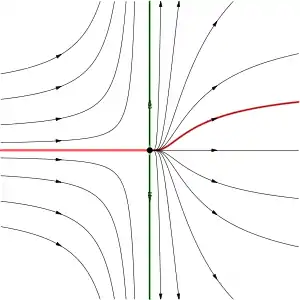
Consider the system

{\dot {x}}=x^{2},\quad {\dot {y}}=y.

The unstable manifold at the origin is the y axis, and the stable manifold is the trivial set {(0, 0)}. Any orbit not on the stable manifold satisfies an equation of the form $y=Ae^{-1/x}$ for some real constant A. It follows that for any real A, we can create a center manifold by piecing together the curve $y=Ae^{-1/x}$ for x > 0 with the negative x axis (including the origin). Moreover, all center manifolds have this potential non-uniqueness, although often the non-uniqueness only occurs in unphysical complex values of the variables.

Delay differential equations often have Hopf bifurcations

Another example shows how a center manifold models the Hopf bifurcation that occurs for parameter $a\approx 4$ in the delay differential equation ${dx}/{dt}=-ax(t-1)-2x^{2}-x^{3}$ . Strictly, the delay makes this DE infinite-dimensional.

Fortunately, we may approximate such delays by the following trick that keeps the dimensionality finite. Define $u_{1}(t)=x(t)$ and approximate the time-delayed variable, $x(t-1)\approx u_{3}(t)$ , by using the intermediaries ${du_{2}}/{dt}=2(u_{1}-u_{2})$ and ${du_{3}}/{dt}=2(u_{2}-u_{3})$ .

For parameter near critical, $a=4+\alpha$ , the delay differential equation is then approximated by the system

{\frac {d{\textbf {u}}}{dt}}=\left[{\begin{array}{ccc}0&0&-4\\2&-2&0\\0&2&-2\end{array}}\right]{\textbf {u}}+\left[{\begin{array}{c}-\alpha u_{3}-2u_{1}^{2}-u_{1}^{3}\\0\\0\end{array}}\right].

Copying and pasting the appropriate entries, the web service finds that in terms of a complex amplitude $s(t)$ and its complex conjugate ${\bar {s}}(t)$ , the center manifold

{\textbf {u}}=\left[{\begin{array}{c}e^{i2t}s+e^{-i2t}{\bar {s}}\\{\frac {1-i}{2}}e^{i2t}s+{\frac {1+i}{2}}e^{-i2t}{\bar {s}}\\-{\frac {i}{2}}e^{i2t}s+{\frac {i}{2}}e^{-i2t}{\bar {s}}\end{array}}\right]+{O}(\alpha +|s|^{2})

and the evolution on the center manifold is

{\frac {ds}{dt}}=\left[{\frac {1+2i}{10}}\alpha s-{\frac {3+16i}{15}}|s|^{2}s\right]+{O}(\alpha ^{2}+|s|^{4})

This evolution shows the origin is linearly unstable for $\alpha >0\ (a>4)$ , but the cubic nonlinearity then stabilises nearby limit cycles as in classic Hopf bifurcation.

Notes

Roberts, A.J. (1993). "The invariant manifold of beam deformations. Part 1: the simple circular rod". J. Elas. 30: 1–54. doi:10.1007/BF00041769.
Carr, Jack (1981). Applications of centre manifold theory. Applied Mathematical Sciences. 35. Springer-Verlag. doi:10.1007/978-1-4612-5929-9. ISBN 978-0-387-90577-8.
Kelley, A. (1967). "The stable, center-stable, center, center-unstable and unstable manifolds". J. Differential Equations. 3 (4): 546–570. Bibcode:1967JDE.....3..546K. doi:10.1016/0022-0396(67)90016-2.
Guckenheimer & Holmes (1997), Section 3.2
Guckenheimer & Holmes (1997), Theorem 3.2.1
Murdock, James (2003). Normal forms and unfoldings for local dynamical systems. Springer-Verlag.
Iooss, G.; Adelmeyer, M. (1992). Topics in Bifurcation Theory. p. 7.
Roberts, A. J. (1988). "The application of centre manifold theory to the evolution of systems which vary slowly in space". J. Austral. Math. Soc. B. 29 (4): 480–500. doi:10.1017/S0334270000005968.
Aulbach, B.; Wanner, T. (1996). "Integral manifolds for Caratheodory type differential equations in Banach spaces". In Aulbach, B.; Colonius, F. (eds.). Six Lectures on Dynamical Systems. Singapore: World Scientific. pp. 45–119.
Aulbach, B.; Wanner, T. (1999). "Invariant foliations for Caratheodory type differential equations in Banach spaces". In Lakshmikantham, V.; Martynyuk, A. A. (eds.). Advances of Stability Theory at the End of XX Century. Gordon & Breach.
Aulbach, B.; Wanner, T. (2000). "The Hartman–Grobman theorem for Caratheodory-type differential equations in Banach spaces". Nonlinear Analysis. 40: 91–104. doi:10.1016/S0362-546X(00)85006-3.
Potzsche, C.; Rasmussen, M. (2006). "Taylor approximation of integral manifolds". Journal of Dynamics and Differential Equations. 18 (2): 427–460. Bibcode:2006JDDE...18..427P. doi:10.1007/s10884-006-9011-8.
Roberts, A.J. (2019). "Backwards theory supports modelling via invariant manifolds for non-autonomous dynamical systems". arXiv:1804.06998 [math.DS].
Hochs, Peter; Roberts, A.J. (2019). "Normal forms and invariant manifolds for nonlinear, non-autonomous PDEs, viewed as ODEs in infinite dimensions". J. Differential Equations. 267 (12): 7263–7312. arXiv:1906.04420. Bibcode:2019JDE...267.7263H. doi:10.1016/j.jde.2019.07.021.
A.J. Roberts (2008). "Normal form transforms separate slow and fast modes in stochastic dynamical systems". Physica A. 387 (1): 12–38. arXiv:math/0701623. Bibcode:2008PhyA..387...12R. doi:10.1016/j.physa.2007.08.023.
A.J. Roberts (1997). "Low-dimensional modelling of dynamics via computer algebra". Comput. Phys. Commun. 100 (3): 215–230. arXiv:chao-dyn/9604012. Bibcode:1997CoPhC.100..215R. doi:10.1016/S0010-4655(96)00162-2.

References

Guckenheimer, John; Holmes, Philip (1997), Nonlinear Oscillations, Dynamical Systems, and Bifurcations of Vector Fields, Applied Mathematical Sciences, 42, Berlin, New York: Springer-Verlag, ISBN 978-0-387-90819-9, corrected fifth printing.

External links

Jack Carr (ed.). "Center manifold". Scholarpedia.

This article is issued from Wikipedia. The text is licensed under Creative Commons - Attribution - Sharealike. Additional terms may apply for the media files.

[Roberts93-1] Roberts, A.J. (1993). "The invariant manifold of beam deformations. Part 1: the simple circular rod". J. Elas. 30: 1–54. doi:10.1007/BF00041769.

[Carr81-2] Carr, Jack (1981). Applications of centre manifold theory. Applied Mathematical Sciences. 35. Springer-Verlag. doi:10.1007/978-1-4612-5929-9. ISBN 978-0-387-90577-8.

[Kelley67b-3] Kelley, A. (1967). "The stable, center-stable, center, center-unstable and unstable manifolds". J. Differential Equations. 3 (4): 546–570. Bibcode:1967JDE.....3..546K. doi:10.1016/0022-0396(67)90016-2.

[4] Guckenheimer & Holmes (1997), Section 3.2

[5] Guckenheimer & Holmes (1997), Theorem 3.2.1

[6] Murdock, James (2003). Normal forms and unfoldings for local dynamical systems. Springer-Verlag.

[7] Iooss, G.; Adelmeyer, M. (1992). Topics in Bifurcation Theory. p. 7.

[8] Roberts, A. J. (1988). "The application of centre manifold theory to the evolution of systems which vary slowly in space". J. Austral. Math. Soc. B. 29 (4): 480–500. doi:10.1017/S0334270000005968.

[9] Aulbach, B.; Wanner, T. (1996). "Integral manifolds for Caratheodory type differential equations in Banach spaces". In Aulbach, B.; Colonius, F. (eds.). Six Lectures on Dynamical Systems. Singapore: World Scientific. pp. 45–119.

[10] Aulbach, B.; Wanner, T. (1999). "Invariant foliations for Caratheodory type differential equations in Banach spaces". In Lakshmikantham, V.; Martynyuk, A. A. (eds.). Advances of Stability Theory at the End of XX Century. Gordon & Breach.

[11] Aulbach, B.; Wanner, T. (2000). "The Hartman–Grobman theorem for Caratheodory-type differential equations in Banach spaces". Nonlinear Analysis. 40: 91–104. doi:10.1016/S0362-546X(00)85006-3.

[12] Potzsche, C.; Rasmussen, M. (2006). "Taylor approximation of integral manifolds". Journal of Dynamics and Differential Equations. 18 (2): 427–460. Bibcode:2006JDDE...18..427P. doi:10.1007/s10884-006-9011-8.

[Roberts2018a-13] Roberts, A.J. (2019). "Backwards theory supports modelling via invariant manifolds for non-autonomous dynamical systems". arXiv:1804.06998 [math.DS].

[14] Hochs, Peter; Roberts, A.J. (2019). "Normal forms and invariant manifolds for nonlinear, non-autonomous PDEs, viewed as ODEs in infinite dimensions". J. Differential Equations. 267 (12): 7263–7312. arXiv:1906.04420. Bibcode:2019JDE...267.7263H. doi:10.1016/j.jde.2019.07.021.

[15] A.J. Roberts (2008). "Normal form transforms separate slow and fast modes in stochastic dynamical systems". Physica A. 387 (1): 12–38. arXiv:math/0701623. Bibcode:2008PhyA..387...12R. doi:10.1016/j.physa.2007.08.023.

[16] A.J. Roberts (1997). "Low-dimensional modelling of dynamics via computer algebra". Comput. Phys. Commun. 100 (3): 215–230. arXiv:chao-dyn/9604012. Bibcode:1997CoPhC.100..215R. doi:10.1016/S0010-4655(96)00162-2.