Centripetal Catmull–Rom spline

Barry and Goldman's pyramidal formulation

Knot parameterization for the Catmull–Rom algorithm

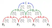
Let ${\displaystyle \mathbf {P} _{i}=[x_{i}\quad y_{i}]^{T}}$ denote a point. For a curve segment ${\displaystyle \mathbf {C} }$ defined by points ${\displaystyle \mathbf {P} _{0},\mathbf {P} _{1},\mathbf {P} _{2},\mathbf {P} _{3}}$ and knot sequence ${\displaystyle t_{0},t_{1},t_{2},t_{3}}$, the centripetal Catmull–Rom spline can be produced by:

${\displaystyle \mathbf {C} ={\frac {t_{2}-t}{t_{2}-t_{1}}}\mathbf {B} _{1}+{\frac {t-t_{1}}{t_{2}-t_{1}}}\mathbf {B} _{2}}$

where

${\displaystyle \mathbf {B} _{1}={\frac {t_{2}-t}{t_{2}-t_{0}}}\mathbf {A} _{1}+{\frac {t-t_{0}}{t_{2}-t_{0}}}\mathbf {A} _{2}}$

${\displaystyle \mathbf {B} _{2}={\frac {t_{3}-t}{t_{3}-t_{1}}}\mathbf {A} _{2}+{\frac {t-t_{1}}{t_{3}-t_{1}}}\mathbf {A} _{3}}$

${\displaystyle \mathbf {A} _{1}={\frac {t_{1}-t}{t_{1}-t_{0}}}\mathbf {P} _{0}+{\frac {t-t_{0}}{t_{1}-t_{0}}}\mathbf {P} _{1}}$

${\displaystyle \mathbf {A} _{2}={\frac {t_{2}-t}{t_{2}-t_{1}}}\mathbf {P} _{1}+{\frac {t-t_{1}}{t_{2}-t_{1}}}\mathbf {P} _{2}}$

${\displaystyle \mathbf {A} _{3}={\frac {t_{3}-t}{t_{3}-t_{2}}}\mathbf {P} _{2}+{\frac {t-t_{2}}{t_{3}-t_{2}}}\mathbf {P} _{3}}$

and

${\displaystyle t_{i+1}=\left[{\sqrt {(x_{i+1}-x_{i})^{2}+(y_{i+1}-y_{i})^{2}}}\right]^{\alpha }+t_{i}}$

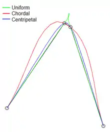
in which ${\displaystyle \alpha }$ ranges from 0 to 1 for knot parameterization, and ${\displaystyle i=0,1,2,3}$ with ${\displaystyle t_{0}=0}$. For centripetal Catmull–Rom spline, the value of ${\displaystyle \alpha }$ is ${\displaystyle 0.5}$. When ${\displaystyle \alpha =0}$, the resulting curve is the standard uniform Catmull–Rom spline; when ${\displaystyle \alpha =1}$, the product is a chordal Catmull–Rom spline.

Gif animation for uniform, centripetal and chordal parameterization of Catmull–Rom spline depending on the α value

Plugging ${\displaystyle t=t_{1}}$ into the spline equations ${\displaystyle \mathbf {A} _{1},\mathbf {A} _{2},\mathbf {A} _{3},\mathbf {B} _{1},\mathbf {B} _{2},}$ and ${\displaystyle \mathbf {C} }$ shows that the value of the spline curve at ${\displaystyle t_{1}}$ is ${\displaystyle \mathbf {C} =\mathbf {P} _{1}}$. Similarly, substituting ${\displaystyle t=t_{2}}$ into the spline equations shows that ${\displaystyle \mathbf {C} =\mathbf {P} _{2}}$ at ${\displaystyle t_{2}}$. This is true independent of the value of ${\displaystyle \alpha }$ since the equation for ${\displaystyle t_{i+1}}$ is not needed to calculate the value of ${\displaystyle \mathbf {C} }$ at points ${\displaystyle t_{1}}$ and ${\displaystyle t_{2}}$.

3D centripetal Catmull-Rom spline segment.

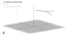
The extension to 3D points is simply achieved by considering ${\displaystyle \mathbf {P} _{i}=[x_{i}\quad y_{i}\quad z_{i}]^{T}}$a generic 3D point ${\displaystyle \mathbf {P} _{i}}$ and

${\displaystyle t_{i+1}=\left[{\sqrt {(x_{i+1}-x_{i})^{2}+(y_{i+1}-y_{i})^{2}+(z_{i+1}-z_{i})^{2}}}\right]^{\alpha }+t_{i}}$

Centripetal Catmull–Rom spline has several desirable mathematical properties compared to the original and the other types of Catmull-Rom formulation.[3] First, it will not form loop or self-intersection within a curve segment. Second, cusp will never occur within a curve segment. Third, it follows the control points more tightly.

In this figure, there is a self-intersection/loop on the uniform Catmull-Rom spline (green), whereas for chordal Catmull-Rom spline (red), the curve does not follow tightly through the control points.

In computer vision, centripetal Catmull-Rom spline has been used to formulate an active model for segmentation. The method is termed active spline model.[4] The model is devised on the basis of active shape model, but uses centripetal Catmull-Rom spline to join two successive points (active shape model uses simple straight line), so that the total number of points necessary to depict a shape is less. The use of centripetal Catmull-Rom spline makes the training of a shape model much simpler, and it enables a better way to edit a contour after segmentation.

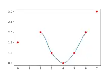
The following is an implementation of the Catmull–Rom spline in Python that produces the plot shown beneath.

import numpy
import matplotlib.pyplot as plt

def CatmullRomSpline(P0, P1, P2, P3, nPoints=100):
    """
    P0, P1, P2, and P3 should be (x,y) point pairs that define the Catmull-Rom spline.
    nPoints is the number of points to include in this curve segment.
    """
    # Convert the points to numpy so that we can do array multiplication
    P0, P1, P2, P3 = map(numpy.array, [P0, P1, P2, P3])

    # Parametric constant: 0.5 for the centripetal spline, 0.0 for the uniform spline, 1.0 for the chordal spline.
    alpha = 0.5
    # Premultiplied power constant for the following tj() function.
    alpha = alpha/2
    def tj(ti, Pi, Pj):
        xi, yi = Pi
        xj, yj = Pj
        return ((xj-xi)**2 + (yj-yi)**2)**alpha + ti

    # Calculate t0 to t4
    t0 = 0
    t1 = tj(t0, P0, P1)
    t2 = tj(t1, P1, P2)
    t3 = tj(t2, P2, P3)

    # Only calculate points between P1 and P2
    t = numpy.linspace(t1, t2, nPoints)

    # Reshape so that we can multiply by the points P0 to P3
    # and get a point for each value of t.
    t = t.reshape(len(t), 1)
    print(t)
    A1 = (t1-t)/(t1-t0)*P0 + (t-t0)/(t1-t0)*P1
    A2 = (t2-t)/(t2-t1)*P1 + (t-t1)/(t2-t1)*P2
    A3 = (t3-t)/(t3-t2)*P2 + (t-t2)/(t3-t2)*P3
    print(A1)
    print(A2)
    print(A3)
    B1 = (t2-t)/(t2-t0)*A1 + (t-t0)/(t2-t0)*A2
    B2 = (t3-t)/(t3-t1)*A2 + (t-t1)/(t3-t1)*A3

    C = (t2-t)/(t2-t1)*B1 + (t-t1)/(t2-t1)*B2
    return C

def CatmullRomChain(P):
    """
    Calculate Catmull–Rom for a chain of points and return the combined curve.
    """
    sz = len(P)

    # The curve C will contain an array of (x, y) points.
    C = []
    for i in range(sz-3):
        c = CatmullRomSpline(P[i], P[i+1], P[i+2], P[i+3])
        C.extend(c)

    return C

# Define a set of points for curve to go through
Points = [[0, 1.5], [2, 2], [3, 1], [4, 0.5], [5, 1], [6, 2], [7, 3]]

# Calculate the Catmull-Rom splines through the points
c = CatmullRomChain(Points)

# Convert the Catmull-Rom curve points into x and y arrays and plot
x, y = zip(*c)
plt.plot(x, y)

# Plot the control points
px, py = zip(*Points)
plt.plot(px, py, 'or')

plt.show()

Plot obtained by the Python example code given above

using UnityEngine;
using System.Collections;
using System.Collections.Generic;

public class Catmul : MonoBehaviour {

	// Use the transforms of GameObjects in 3d space as your points or define array with desired points
	public Transform[] points;
	
	// Store points on the Catmull curve so we can visualize them
	List<Vector2> newPoints = new List<Vector2>();
	
	// How many points you want on the curve
	uint numberOfPoints = 10;
	
	// Parametric constant: 0.0 for the uniform spline, 0.5 for the centripetal spline, 1.0 for the chordal spline
	public float alpha = 0.5f;
	
	/////////////////////////////
	
	void Update()
	{
	    CatmulRom();
	}
	
	void CatmulRom()
	{
		newPoints.Clear();

		Vector2 p0 = points[0].position; // Vector3 has an implicit conversion to Vector2
		Vector2 p1 = points[1].position;
		Vector2 p2 = points[2].position;
		Vector2 p3 = points[3].position;

		float t0 = 0.0f;
		float t1 = GetT(t0, p0, p1);
		float t2 = GetT(t1, p1, p2);
		float t3 = GetT(t2, p2, p3);

		for (float t=t1; t<t2; t+=((t2-t1)/(float)numberOfPoints))
		{
		    Vector2 A1 = (t1-t)/(t1-t0)*p0 + (t-t0)/(t1-t0)*p1;
		    Vector2 A2 = (t2-t)/(t2-t1)*p1 + (t-t1)/(t2-t1)*p2;
		    Vector2 A3 = (t3-t)/(t3-t2)*p2 + (t-t2)/(t3-t2)*p3;
		    
		    Vector2 B1 = (t2-t)/(t2-t0)*A1 + (t-t0)/(t2-t0)*A2;
		    Vector2 B2 = (t3-t)/(t3-t1)*A2 + (t-t1)/(t3-t1)*A3;
		    
		    Vector2 C = (t2-t)/(t2-t1)*B1 + (t-t1)/(t2-t1)*B2;
		    
		    newPoints.Add(C);
		}
	}

	float GetT(float t, Vector2 p0, Vector2 p1)
	{
	    float a = Mathf.Pow((p1.x-p0.x), 2.0f) + Mathf.Pow((p1.y-p0.y), 2.0f);
	    float b = Mathf.Pow(a, alpha * 0.5f);
	   
	    return (b + t);
	}
	
	// Visualize the points
	void OnDrawGizmos()
	{
	    Gizmos.color = Color.red;
	    foreach (Vector2 temp in newPoints)
	    {
	        Vector3 pos = new Vector3(temp.x, temp.y, 0);
	        Gizmos.DrawSphere(pos, 0.3f);
	    }
	}
}

For an implementation in 3D space, after converting Vector2 to Vector3 points, the first line of function GetT should be changed to this: Mathf.Pow((p1.x-p0.x), 2.0f) + Mathf.Pow((p1.y-p0.y), 2.0f) + Mathf.Pow((p1.z-p0.z), 2.0f);

• Cubic Hermite splines

• Catmull-Rom curve with no cusps and no self-intersections – implementation in Java
• Catmull-Rom curve with no cusps and no self-intersections – simplified implementation in C++
• Catmull-Rom splines – interactive generation via Python, in a Jupyter notebook

References

- Catmull, Edwin; Rom, Raphael (1974). "A class of local interpolating splines". In Barnhill, Robert E.; Riesenfeld, Richard F. (eds.). Computer Aided Geometric Design. pp. 317–326. doi:10.1016/B978-0-12-079050-0.50020-5. ISBN 978-0-12-079050-0.
- Barry, Phillip J.; Goldman, Ronald N. (August 1988). A recursive evaluation algorithm for a class of Catmull–Rom splines. Proceedings of the 15st Annual Conference on Computer Graphics and Interactive Techniques, SIGGRAPH 1988. 22. Association for Computing Machinery. pp. 199–204. doi:10.1145/378456.378511.
- Yuksel, Cem; Schaefer, Scott; Keyser, John (July 2011). "Parameterization and applications of Catmull-Rom curves". Computer-Aided Design. 43 (7): 747–755. CiteSeerX 10.1.1.359.9148. doi:10.1016/j.cad.2010.08.008.
- Jen Hong, Tan; Acharya, U. Rajendra (2014). "Active spline model: A shape based model-interactive segmentation" (PDF). Digital Signal Processing. 35: 64–74. arXiv:1402.6387. doi:10.1016/j.dsp.2014.09.002. S2CID 6953844.
External links