Distance sampling

Distance sampling is a widely used group of closely related methods for estimating the density and/or abundance of populations. The main methods are based on line transects or point transects.[1][2] In this method of sampling, the data collected are the distances of the objects being surveyed from these randomly placed lines or points, and the objective is to estimate the average density of the objects within a region.[3]

Basic line transect methodology

Basic distance sampling survey approach using line transects. A field observer detects an object and records distance r and angle θ to the transect line. This allows calculation of object distance to the transect (x). All x from the survey are used to model how detectability decreases with distance from the transect, which allows estimation of total population density in the surveyed area.

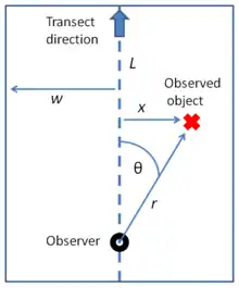
A common approach to distance sampling is the use of line transects. The observer traverses a straight line (placed randomly or following some planned distribution). Whenever they observe an object of interest (e.g., an animal of the type being surveyed), they record the distance from their current position to the object (r), as well as the angle of the detection to the transect line (θ). The distance of the object to the transect can then be calculated as x = r * sin(θ). These distances x are the detection distances that will be analyzed in further modeling.

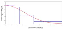
Objects are detected out to a pre-determined maximum detection distance w. Not all objects within w will be detected, but a fundamental assumption is that all objects at zero distance (i.e., on the line itself) are detected. Overall detection probability is thus expected to be 1 on the line, and to decrease with increasing distance from the line. The distribution of the observed distances is used to estimate a "detection function" that describes the probability of detecting an object at a given distance. Given that various basic assumptions hold, this function allows the estimation of the average probability P of detecting an object given that is within width w of the line. Object density can then be estimated as $D = n / (P * a)$ , where n is the number of objects detected and a is the size of the region covered (total length of the transect (L) multiplied by 2w).

In summary, modeling how detectability drops off with increasing distance from the transect allows estimating how many objects there are in total in the area of interest, based on the number that were actually observed.[2]

The survey methodology for point transects is slightly different. In this case, the observer remains stationary, the survey ends not when the end of the transect is reached but after a pre-determined time, and measured distances to the observer are used directly without conversion to transverse distances. Detection function types and fitting are also different to some degree.[2]

Detection function

Half-normal detection function (red line) fitted to PDF of detection data. Data have been collated into distance bands (either collected as such, or combined after collection to improve model fitting). Detection probability decreases with distance from center line (y = 0).

The drop-off of detectability with increasing distance from the transect line is modeled using a detection function g(y) (here y is distance from the line). This function is fitted to the distribution of detection ranges represented as a probability density function (PDF). The PDF is a histogram of collected distances and describes the probability that an object at distance y will be detected by an observer on the center line, with detections on the line itself (y = 0) assumed to be certain (P = 1).

By preference, g(y) is a robust function that can represent data with unclear or weakly defined distribution characteristics, as is frequently the case in field data. Several types of functions are commonly used, depending on the general shape of the detection data's PDF:

Detection function	Form
Uniform	$1/ w$
Half-normal	$exp(- y 2 /2 σ 2)$
Hazard-rate	$1-exp(-(y / σ) -b)$
Negative exponential	$exp(- ay)$

Here w is the overall detection truncation distance and a, b and σ are function-specific parameters. The half-normal and hazard-rate functions are generally considered to be most likely to represent field data that was collected under well-controlled conditions. Detection probability appearing to increase or remain constant with distance from the transect line may indicate problems with data collection or survey design.[2]

Series expansions

A frequently used method to improve the fit of the detection function to the data is the use of series expansions. Here, the function is split into a "key" part (of the type covered above) and a "series" part; i.e., g(y) = key(y)[1 + series(y)]. The series generally takes the form of a polynomial (e.g. a Hermite polynomial) and is intended to add flexibility to the form of the key function, allowing it to fit more closely to the data PDF. While this can improve the precision of density/abundance estimates, its use is only defensible if the data set is of sufficient size and quality to represent a reliable estimate of detection distance distribution. Otherwise there is a risk of overfitting the data and allowing non-representative characteristics of the data set to bias the fitting process.[2][4]

Assumptions and sources of bias

Since distance sampling is a comparatively complex survey method, the reliability of model results depends on meeting a number of basic assumptions. The most fundamental ones are listed below. Data derived from surveys that violate one or more of these assumptions can frequently, but not always, be corrected to some extent before or during analysis.[1][2]

Basic assumptions of distance sampling
Assumption	Violation	Prevention/post-hoc correction	Data example
All animals on the transect line itself are detected (i.e., P(0) = 1)	This can often be assumed in terrestrial surveys, but may be problematic in shipboard surveys. Violation may result in strong bias of model estimates	In dual observer surveys, one observer may be tasked to "guard the centerline". Post-hoc fixes are sometimes possible but can be complex.[1] It is thus worth avoiding any violations of this assumption
Animals are randomly and evenly distributed throughout the surveyed area	The main sources of bias are a) clustered populations (flocks etc.) but individual detections are treated as independent b) transects are not placed independently of gradients of density (roads, watercourses etc.) c) transects are too close together	a) record not individuals but clusters + cluster size, then incorporate estimation of cluster size into the detection function b) place transects either randomly, or across known gradients of density c) make sure that maximum detection range (w) does not overlap between transects
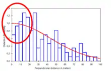
Animals do not move before detection	Resulting bias is negligible if movement is random. Movement in response to the observer (avoidance/attraction) will incur a negative/positive bias in detectability	Avoidance behaviour is common and may be difficult to prevent in the field. An effective post-hoc remedy is the averaging-out of data by partitioning detections into intervals, and by using detection functions with a shoulder (e.g., hazard-rate)	An indication of avoidance behaviour in the data - detections initially increase rather than decrease with added distance to the transect line
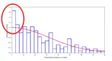
Measurements (angles and distances) are exact	Random errors are negligible, but systematic errors may introduce bias. This often happens with rounding of angles or distances to preferred ("round") values, resulting in heaping at particular values. Rounding of angles to zero is particularly common	Avoid dead reckoning in the field by using range finders and angle boards. Post-hoc smoothing of data by partitioning into detection intervals is effective in addressing minor biases	An indication of angle rounding to zero in the data - there are more detections than expected in the very first data interval

References

Buckland, S. T., Anderson, D. R., Burnham, K. P. and Laake, J. L. (1993). Distance Sampling: Estimating Abundance of Biological Populations. London: Chapman and Hall. ISBN 0-412-42660-9
Buckland, Stephen T.; Anderson, David R.; Burnham, Kenneth Paul; Laake, Jeffrey Lee; Borchers, David Louis; Thomas, Leonard (2001). Introduction to distance sampling: estimating abundance of biological populations. Oxford: Oxford University Press.
Everitt, B. S. (2002) The Cambridge Dictionary of Statistics, 2nd Edition. CUP ISBN 0-521-81099-X (entry for distance sampling)
Buckland, S. T. (2004). Advanced distance sampling. Oxford University Press.

External links

Bibliography of > 1400 scientific publications using the method

This article is issued from Wikipedia. The text is licensed under Creative Commons - Attribution - Sharealike. Additional terms may apply for the media files.

[buckland1993-1] Buckland, S. T., Anderson, D. R., Burnham, K. P. and Laake, J. L. (1993). Distance Sampling: Estimating Abundance of Biological Populations. London: Chapman and Hall. ISBN 0-412-42660-9

[buckland2001-2] Buckland, Stephen T.; Anderson, David R.; Burnham, Kenneth Paul; Laake, Jeffrey Lee; Borchers, David Louis; Thomas, Leonard (2001). Introduction to distance sampling: estimating abundance of biological populations. Oxford: Oxford University Press.

[3] Everitt, B. S. (2002) The Cambridge Dictionary of Statistics, 2nd Edition. CUP ISBN 0-521-81099-X (entry for distance sampling)

[buckland2004-4] Buckland, S. T. (2004). Advanced distance sampling. Oxford University Press.