Facet theory
Facet theory is a metatheory for the multivariate behavioral sciences that posits that replicable research and meaningful measurements can be advanced by discovering relationships between classifications of observations and partitions of suitable data-representation spaces. These spaces may depict either similarity measures (e.g., correlations) or partially ordered sets, derived from the data.
Facet Theory was initiated by Louis Guttman[1] and has been further developed and applied in a variety of disciplines of the behavioral sciences including psychology, sociology, and business administration.
Variables as statistical units. Facet theory acknowledges that, in behavioral research, observed variables typically form but a sample from an infinite number, or a very large number of variables that make up the investigated attribute (the content universe). Consequently, facet theory proposes techniques for sampling variables for observation from the entire content universe; and for making inferences, from the sample of observed variables to the entire content universe, as follows:
(a) Sampling variables from the content universe. This is done with the aid of a mapping sentence, essentially a function whose domain consists of the respondents and of the stimuli as arguments, and whose image consists of the cartesian product of the ranges of responses to the stimuli, where each response-range is similarly ordered from high to low with respect to a concept common to all stimuli. When stimuli are classified a priori by one or more content criteria, the mapping sentence facilitates stratified sampling of content universe. See Section 1 below.
A classification of the stimuli by their content is called a content facet; and the pre-specified set of responses to a stimulus (classifying respondents by their response to that stimulus) is called a range facet.
(b) Making inferences from the sample of observed variables to the entire content universe. Such inferences require a specification of the kind of research-outcomes with respect to which inferences are to be made. Facet theory posits that scientifically stable (reproducible) outcomes would result from regional hypotheses; hypotheses about correspondences between the definitional (content- or range-) facets on the one hand, and empirical partitionings into regions of certain geometric spaces, on the other hand. Thus, a regional hypothesis specifies a one-to-one correspondence between facet-elements (classes) and disjoint regions in space.
Of the many types of spaces that have been proposed,[2] two stand out as especially fruitful:
- Faceted-SSA (Faceted Smallest Space Analysis).[3][4] In the geometric space produced by this procedure, variables are mapped as points, subject to the condition: If rij > rkl then dij ≤ dkl, where rij is a measure of similarity between variable i and j (often the correlation coefficients between variables); and dij is the distance between their points in space. The investigated universe, defined as the totality of its variables, is represented by a connected subset of the geometric space, often referred to as the SSA map. For each content facet, a 1-1 correspondence is then sought between its elements and a region in the SSA map. A regional hypothesis anticipates that a simple partition of the space can be found, such that each of its regions would include the variables of just one of the classes specified by the content facet. Faceted SSA is the basis for structuring the investigated attribute. See Section 2 below.
- POSAC (Partial Order Scalogram Analysis by base Coordinates).[5] This procedure is based on the analysis of respondents with respect to a partial order relationship that exists between them. Thus, it is assumed that every pair of respondents, pi, pj, is either comparable (designated by pi S pj), with one of them greater or equal to the other (pi ≥ pj) with respect to the observed attribute; or they are incomparable (designated by pi $ pj ) with respect to that attribute. POSAC aims to represent respondents pi as points x1(pi) … xm(pi) in the smallest m-coordinates space, X, whose coordinates preserve observed partial order relations (comparability and incomparability). That is, pi$pj iff there exist two coordinates xs, xt for which the following holds: xs(pi) > xs(pj) but xt(pi) < xt(pj). For each range facet, a 1-1 correspondence is then sought between its elements (scores) and a partition of the POSAC space into allowable regions, those that are separated by non-increasing hyperplanes; e.g., non-increasing lines, in the 2-dimensional case. POSAC is the basis for multiple scaling measurements of the investigated attribute. See Section 3 below.
This article continues with Section 1 describing the mapping sentence device for formally defining the system of observations, for providing the terms in which hypotheses may be formulated, and for facilitating the stratified sampling of variables. Section 2 outlines facet theory's foundations as applied to its use of similarity representation spaces (Faceted Smallest Space Analysis, Faceted SSA), and illustrates them with an example from intelligence research. Section 3 outlines facet theory's foundations as applied to its use of coordinate space representation of partially ordered sets (Multiple Scaling by Partial Order Scalogram Analysis with Coordinates, POSAC), and illustrates them with a theory-based measurements of distributive justice attitudes. Section 4 concludes with some comments on facet theory including its comparison to factor analysis.
The mapping sentence
The mapping sentence is a semantic device for defining and communicating the system of observations to be performed in a particular research. As such, the mapping sentence provides also the essential concepts in terms of which research hypotheses may be formulated.
An example from intelligence research
Suppose members pi of a population P are observed with respect to their success in a written verbal intelligence test. Such observations may be described as a mapping from the observed population to the set of possible scores, say, R = {1,…,10}: Pq1 → R, where q1 is the sense in which a specific score is assigned to every individual in the observed population P, i.e., q1 is "verbal intelligence" in this example. Now, one may be interested in observing also the mathematical or, more specifically, the numerical intelligence of the investigated population; and possibly also their spatial intelligence. Each of these kinds of intelligence is a "sense" in which population members pi may be mapped into a range of scores R = {1,…,10}. Thus, 'intelligence' is now differentiated into three types of materials: verbal (q1), numerical (q2) and spatial (q3). Together, P, the population, and Q = {q1, q2, q3}, the set of types of intelligence, form a cartesian product which constitutes the mapping domain. The mapping is from the set of pairs (pi, qj) to the common range of test-scores R = {1,…,10}: P × Q → R.
A facet is a set that serves as a component-set of a cartesian product. Thus, P is called the population facet, Q is called a content facet, and the set of scores obtainable for each test is a range facet. The range facets of the various items (variables) need not be identical in size: they may have any finite number of scores, or categories, greater or equal to 2.
The Common Meaning Range (CMR)
The ranges of the items pertaining to an investigated content-universe – intelligence in this example – should all have a Common Meaning Range (CMR); that is, they must be ordered from high to low with respect to a common meaning. Following Guttman, the common meaning proposed for the ranges of intelligence-items is "correctness with respect to an objective rule".
The concept of CMR is central in facet theory: It serves to define the content-universe being studied by specifying the universe of items pertaining to that content-universe. Thus, the mapping-definition of intelligence, advanced by facet theory is:
"An item belongs to the universe of intelligence items if and only if its domain requires performance of a cognitive task concerning an objective rule and its range is ordered from high correctness to low correctness with respect to that rule."
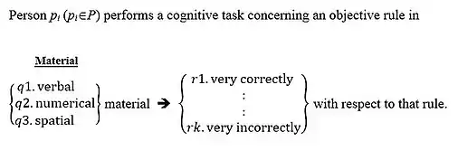
An initial framework for observing intelligence could be Mapping Sentence 1.
The mapping sentence serves as a unified semantic device for specifying the system of intelligence test items, according to the present conceptualization. Its content facet, the material facet, may now serve as a classification of intelligence test items to be considered. Thus, in designing observations, a stratified sampling of items is afforded by ensuring an appropriate selection of items from each of the material facet elements; that is, from each class of items: the verbal, the numerical and the spatial.
Enriching the mapping sentence
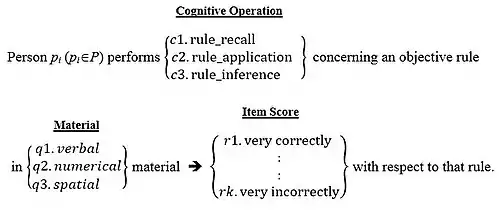
The research design can be enriched by introducing to the mapping sentence an additional, independent classification of the observations in the form of an additional content-facet, thereby facilitating systematic differentiations of the observations. For example, intelligence items may be classified also according to the cognitive operation required in order to respond correctly to an item: whether rule-recall (memory), rule-application, or rule-inference. Instead of the three sub-content-universes of intelligence defined by the material facet alone, we now have nine sub-content-universes defined by the cartesian multiplication of the material and the mental-operation facets. See mapping sentence 2.
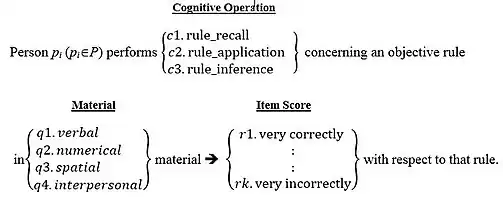
Another way of enriching a mapping sentence (and the scope of the research) is by adding an element (a class) to an existing content facet; for example, by adding Interpersonal material as a new element to the extant material facet. See Mapping Sentence 3.
Content profiles
A selection of one element from each of the two content facets defines a content profile which represents a sub-content-universe of intelligence. For example, the content profile (c2, q2) represents the application of rules for performing mathematical computations, such as performing long division. The 3x4=12 sub-content-universes constitute twelve classes of intelligence items. In designing observations, the researcher would strive to include a number of varied items from each of these 12 classes so that the sample of observed items would be representative of the entire intelligence universe. Of course, this stratified sampling of items depends on the researchers' conception of the studied domain, reflected in their choice of content-facets. But, in the larger cycle of the scientific investigation (which includes Faceted SSA of empirical data, see next section), this conception may undergo adjustments and remolding, converging to improved choices of content-facets and observations, and ultimately to robust theories in research domain. In general, mapping sentences may attain high levels of complexity, size and abstraction through various logical operations such as recursion, twist, decomposition and completion.
Cartesian decomposition and completion: an example
In drafting a mapping sentence, an effort is made to include the most salient content-facets, according to the researcher's existing conception of the investigated domain. And for each content facet, attempt is made to specify its elements (classes) so that they be exhaustive (complete) and exclusive (non-overlapping) of each other. Thus, the element 'interpersonal' has been added to the incumbent 3-element material facet of intelligence by a two-step facet-analytic procedure. Step 1, cartesian decomposition of the 3-element material facet into two binary elementary facets: The Environment Facet, whose elements are 'physical environment' and 'human-environment'; and the Symbolization Facet whose elements are 'symbolic' (or high symbolization), and 'concrete' (or low symbolization). Step 2, cartesian completion of the material facet is then sought by attempting to infer the missing material classifiable as 'human environment' and 'concrete'.
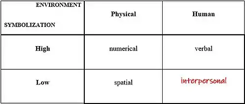
In facet theory, this 2×2 classification of intelligence-testing material may now be formulated as an hypothesis to be tested empirically, using Faceted Smallest Space Analysis (SSA).
Complementary topics concerning the mapping sentence
Despite its seemingly rigid appearance, the mapping sentence format can accommodate complex semantic structures such as twists and recursions, while retaining its essential cartesian structure.[6]
In addition to guiding the collection of data, mapping sentences have been used to content-analyze varieties of conceptualizations and texts—such as organizational quality, legal documents and even dream stories.[7][8]
Concepts as spaces: faceted SSA
Facet theory conceives of a multivariate attribute as a content-universe defined by the set of all its items, as specified by the attribute mapping-definition, illustrated above. In facet-theoretical data analysis, the attribute (e.g., intelligence) is likened to a geometric space of suitable dimensionality, whose points represent all possible items. Observed items are processed by Faceted SSA, a version of Multidmensional Scaling (MDS)[9] which involves the following steps:
- Receiving as input (or computing from input data) a matrix of similarity coefficients, specifying, for each pair of items how similar they are. A common example is the computation of a correlation-coefficient matrix from input data, where the size of a correlation coefficient between two variables reflects the degree of similarity between them.
- Mapping the items (variables) as points in a geometric space of a given dimensionality while preserving as well as possible the condition: If rij>rkl then dij<dkl for all i,j,k,l where rij is the similarity measure (e.g., correlation coefficient) between variables i,j and dij is the distance between their points in the space. Most often, Euclidean distance function (Minkowsky distance of order 2) is used. But other distance functions, especially the Manhattan distance function (Minkowsky distance of order 1) are called for. (See Subsection Relating POSAC Measurement Space to the SSA Concept Space below.) The goodness-of-fit of the resulting mapping may be assessed by a loss function– Kruskal's Stress coefficient[10] or Guttman's Coefficient of Alienation.[3]
- Partitioning the space as well as possible, into simple regions (stripe, sectors or concentric rings) whose variables are in 1-1 correspondence with a pre-conceived content-facet. To run this option, content facet(s) must be specified as Faceted SSA input.
Step 3 of Faceted SSA incorporates the idea that observed variables included in the Faceted SSA procedure, typically constitute a small subset from the countless items that define the attribute content-universe. But their locations in space may serve as clues that guide the partitioning of the space into regions, in effect classifying all points in space, including those pertaining to unobserved items (had they been observed). This procedure, then, tests the regional hypothesis that the sub-content-universes defined by a content-facet elements exist each as a distinct empirical entity. The Shye-Kingsley Separation Index (SI) assesses the goodness-of-fit of the partition to the content-facet.[11]
The spatial scientific imagery suggested by Facet Theory has far reaching consequences that set Facet Theory apart from other statistical procedures and research strategies. Specifically, it facilitates inferences concerning the structure of the entire content-universe investigated, including unobserved items.
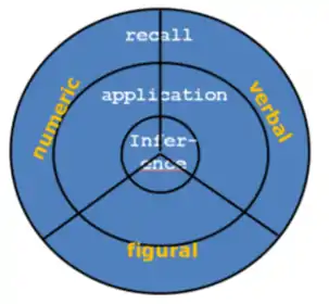
Example 1. The structure of intelligence
Intelligence testing has been conceived as described above, with Mapping Sentence 2 as a framework for its
observation.[12] In many studies, different samples of variables conforming to Mapping Sentence 2 have been analyzed confirming two regional hypotheses:
- The Material Content Facet corresponds to a partition of the Faceted SSA map of intelligence into sectors, each containing the items of a single material — verbal, numeric, and figural (spatial).
- The Cognitive Operation Facet corresponds to a partition of the Faceted SSA map of intelligence into concentric rings, with the innermost ring containing inference items; the middle ring containing the rule-application items; and the outermost ring containing the rule-recall items.
The superposition of these two partition patterns results in a scheme known as the Radex Theory of Intelligence, see Figure 1.
The radex structure, which originated earlier as "a new approach to factor analysis",[13] has been found also in the study of color perception[14] as well as in other domains of research.
Faceted SSA has been applied in a wide variety of research areas including value research[15][16] social work [17] and criminology[18][19] and many others.
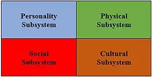
Example 2. The structure of quality of life
The Systemic Quality of Life (SQOL) has been defined as the effective functioning of human individuals in four functioning subsystems: the cultural, the social, the physical and the personality subsystems.[20] The axiomatic foundations of SQOL suggest the regional hypothesis that the four subsystems should be empirically validated (i.e., item of each would occupy a distinct region) and that they be mutually oriented in space in a specific 2x2 pattern topologically equivalent to the 2x2 classification shown in Figure 2 (i.e., personality opposite cultural, and physical opposite social). The hypothesis has been confirmed by many studies.
Types of partition patterns
Of the many possible partitions of a 2-d concept space, three stand out as especially useful for theory construction:
- The Axial Partition Pattern: Partitioning of the space into stripes by parallel lines.
- The Angular (a/k/a polar) Partition Pattern: Partitioning of the space into sectors by radii emanating from a point in space.
- The Radial (a/k/a modular) Partition Pattern: Partitioning of the space into concentric rings by concentric circles.
The advantages of these partition patterns as likely models for behavioral data are that they are describable by a minimal number of parameters, hence avoid overfitting; and that they are generalizable to partition in spaces of higher dimensionalities.
In testing regional hypotheses, the fit of a content-facet to any one of these three models is assessed the Separation Index (SI), a normalized measure of the deviation of variables from the region assigned to them by the model.[11]
Concept spaces in higher dimensionalities have been found as well.[21]
Principles of faceted SSA: A summary
1. The attribute under study is represented by a geometric space.
2. Variables of the attribute are represented as points in that space. Conversely, every point in the geometric space is a variable of the attribute. This is the Continuity Principle.[4]
3. The observed variables, located as points in the empirical Faceted SSA map, constitute but a sample drawn from the many (possibly infinitely many) variables constituting the content universe of the attribute investigated.
4. The observed variables chosen for SSA must all belong to the same content universe. This is ensured by including in the SSA only variables whose ranges are similarly ordered with respect to a common meaning (CMR).
5. The sample of variables marked on the Faceted SSA map is used as a guide for inferring possible partitions of the SSA-attribute-map into distinct regions, each region representing a component, or subdomain, of the attribute.
6. In Facet Theory, relationships between attribute components (such as verbal intelligence and numeric intelligence as components of intelligence), are expressed in geometric terms –such as shapes and spatial orientation – rather than in algebraic terms. Just as one would describe relationships between neighboring countries in terms of their shapes and geographical orientation, not in terms of distances between them.
7. The imagery of an attribute as a continuous space, from which variables are sampled, implies that clustering of variables in SSA map has no significance: It is just an artifact of the sampling of the variables. Sampled variables that are clustered together may belong to different subdomains; just as two cities that are close together may be located in different countries. Conversely, variables that are far apart, may belong to the same sub-domain; just as two cities that are far apart may belong to the same country. What matters is the identification of distinct regions with well-defined sub-domains. Facet Theory proposes a way of transcending accidental clustering of variables by focusing on a robust and replicable aspect of the data, namely the partitionability of the attribute-space.
These principles bring in new concepts, raise new questions, and opens new ways of understanding behavior. Thus, Facet Theory represents a paradigm of its own for multivariate behavioral research.
Complementary topics in faceted SSA
Besides analyzing a data matrix of N individuals by n variables, as discussed above, Faceted SSA is usefully employed in additional modes.
Direct measures of (dis)similarity. For a given a set of objects and a similarity (or dissimilarity) measure between every pair of objects, Faceted SSA can provide a map whose regions correspond to a specified classification of the objects. For example, in a study of color perception, a sample of spectral colors, with a measure of perceived similarity between every pair of colors, yielded the radex theory of spectral color perception.[14] In a study of community elites, a measure of distance devised between pairs of community leaders, yielded a sociometric map whose regions were interpreted from the perspective of sociological theory.[22]
Transposed data matrix. Switching the roles of individuals and variables, Faceted SSA may be applied to individuals rather than to the variables. This rarely used procedure may be justified to the extent variables evenly cover a research domain. For example, intercorrelations between members of a multidisciplinary team of experts were computed based on their human quality-of life value assessments. The resulting Faceted SSA map yielded a radex of disciplines, supporting the association between social institutions and human values.[23]
Multiple scaling by POSAC
In Facet Theory, the measurement of investigated individuals (and, by extension, of all individuals belonging to the sampled population) with respect to a multivariate attribute, is based on the following assumptions and conditions:
- Variables processed by Facet Theory measurement operations to be described below, evenly cover the attribute content universe. To ensure such coverage, Facet Theory measurement operations are often performed not on the sample of the observed items themselves, but rather on composite variables that represent facet elements that had been validated by Faceted SSA.
- The sample of individuals is rich enough to allow existing score-profiles of the processed variables to be observed.
- In the resulting measurement, order relations among individuals should preserve sufficiently well order relations (including comparability and incomparability; see below) between individuals' profiles of the processed variables.
- The result of the measurement operation yields the smallest number of scales;
- The resultant scales represent fundamental variables whose interpretation derives from the contents of the observed items, but does not depend on the particular sample of items observed.
Partial order analysis of observed data. Let observed items v1,...,vn with a common-meaning range (CMR) represent an investigated content universe; let A1,...,An be their ranges with each Aj ordered from high to low with respect to the common meaning; and let A = A1×A2 × ... × An be the cartesian product of all the range facets, Aj (j = 1,...,n). A system of observations is a mapping P → A from the observed subjects P to A, that is, each subject pi gets a score from each Aj (j = 1,...,n), or pi → [ai1,ai2, ..., ain] a(pi). The point a(pi) in A is also called the profile of pi, and the subset A′ of A () of observed profiles is called a scalogram. Facet Theory defines relations between profiles as follows: Two different profiles ai = [ai1,ai2,...,ain] and aj = [aj1,aj2,...,ajn], are comparable, denoted by aiSaj, with ai greater than aj, ai > aj, if and only if aik ≥ ajk for k = 1, ..., n, and aik′ > ajk′ for some k. Two different profiles are incomparable, denoted by ai $ aj, if neither ai > aj nor aj > ai. A, and therefore its subset A′, form a partially ordered set.
Facet Theoretical measurement consists in mapping points a(pi) of A' into a coordinate space X of the lowest dimensionality while preserving observed order relations, including incomparability:
Definition. The p.o. dimensionality of scalogram A' is the smallest m (m ≤ n) for which there exist m facets X1 ... Xm (each Xi is ordered) and there exists a 1-1 mapping Q:X′ → A′ from X′ () to A′ such that a > a′ if and only if x > x′ whenever Q maps points x, x′ in X′ to points a, a′ ∈ A.[5]
The coordinate scales, Xi (i = 1, ..., m) represent underlying fundamental variables whose meanings must be inferred in any specific application. The well known Guttman scale[24] [24] (example: 1111, 1121, 1131, 2131, 2231, 2232) is simply a 1-d scalogram, i.e. one all of whose profiles are comparable.
The procedure of identifying and interpreting the coordinate scales X1...Xm is called multiple scaling. multiple scaling is facilitated by partial order scalogram analysis by base coordinates (POSAC) for which algorithms and computer programs have been devised. In practice, a particular dimensionality is attempted and a solution that best accommodates the order-preserving condition is sought. The POSAC/LSA program finds an optimal solution in 2-d coordinate space, then goes on to analyze by Lattice Space Analysis (LSA) the role played by each of the variables in structuring the POSAC 2-space, thereby facilitating interpretation of the derived coordinate scales, X1, X2. Recent developments include the algorithms for computerized partitioning of the POSAC space by the range facet of each variable, which induces meaningful intervals on the coordinate scales, X, Y.
Example 3. TV watching patterns: analysis of simplified survey data[25]
Members of a particular population were asked four questions: whether they watched TV the night before for an hour at 7 PM (hour 1), at 8 PM (hour 2), at 9 PM (hour 3) and at 10 PM (hour 4). A positive answer to a question was recorded as 1, and a negative answer, as 0. Thus, for example, the profile 1010 represents a person who watched TV at 7 PM and at 9 PM but not at 8 PM and at 10 PM. Suppose that out of the 16 combinatorially possible profiles, only the following eleven profiles were observed empirically: 0000, 1000, 0100, 0010, 0001, 1100, 0110, 0011, 1110, 0111, 1111. Figure 3 is an order-preserving mapping of these profiles into a 2-dimensional coordinate space.
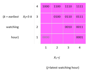
Given this POSAC solution, an attempt is made to interpret the two coordinates, X1 and X2, as two fundamental scales of the investigated phenomenon of evening TV watching by the investigated population. This is done by, first, interpreting the intervals (equivalence classes) within each coordinate, and then trying to conceptualize the derived meanings of the ordered intervals, in terms of a meaningful notion that may be attributed to the coordinate.
In the present simplified example, this is easy: Inspecting the map, we attempt to identify the feature that distinguishes all profiles with given score in X1. Thus, we find that profiles with X1=4, and only they, represent TV watching in the fourth hour. Profiles with X1 = 3 all have 1 in the third watching hour but 0 at the fourth hour, i.e., the third hour is the latest watching hour. X1 = 2 is assigned to, and only to, profiles whose latest watching hour is the second hour. And, finally, X1 = 1 is for the profile 1000 which represents the fact that the first hour is the only – and therefore the latest – watching hour (ignoring the profile 0000 of those who didn’t watch TV at the specified hours, and could be assigned (0,0) in this coordinate-space). Hence, it may be concluded that intervals of coordinate X1 represent j=the latest hour—among the four hours observed—in which TV was watched, (j = 1, …, 4). Similarly, it is found that intervals of coordinate X2 represent 5 − k for k (k = 1, …, 4) is the earliest hour of TV watching.
Indeed, for profiles of the observed set, which represent a single sequence of continuous TV watching, specification of the earliest and latest watching hours, provide full description of the watching hours.
Example 3 illustrates key features of Multiple Scaling by POSAC that render this procedure a theory-based multivariate measurement:
- The two scores assigned by Multiple Scaling to every observed profile—and hence to every person in the observed sample—replace the more numerous scores (four, in the present example) of the observed variables, while retaining all observed order relations, including incomparability. The new scores assess observed persons on the two coordinate-scales, taken to constitute Nature's fundamental variables.
- The two coordinate-scales have intrinsic meanings that probe into a deeper significance than the observed variables considered severally. In the present example, the earliest and the latest hour indeed exhaust the essential aspects of the pattern of TV watching, given the particular set of observed profiles.
- The concepts derived for the fundamental, unobserved coordinate-scales retain the CMR—the essential meaning common to all observed variables. In the present example, the CMR is more (vs. less) TV watching. For, considering the observed variables, each of them records high (1) vs. low (0) TV watching in a given hour. And the derived coordinate-scales, too, record high (4) vs. low (1) TV watching, since ceteris paribus, the later is the latest watching hour, the more TV one watches (X1); and the earlier is the earliest watching hour, the more TV one watches ( X2).
These features are present also in applications that are less obvious, to produce scales with novel meanings.
Example 4. Measuring distributive justice attitudes
In the systemic theory of distributive justice (DJ), alternative allocations of a given amount of an educational resource (100 supplementary teaching hours) between gifted and disadvantaged pupils, may be classified by one of four types, the preference for each reflecting one's DJ attitude:[26]
Equality, where the gifted and the disadvantaged pupils get the same amount of the supplementary resource;
Fairness, where the disadvantaged pupils get more of the resource than the gifted, in proportion to their weakness relative to the gifted;
Utility, where the gifted get more of the resource than the disadvantaged pupils (so as to promote future contribution to the general good);
Corrective Action, where the disadvantaged pupils get more of the resource than the gifted over and above the proportion of their weakness relative to the gifted pupils, (so as to compensate them for past accumulated disadvantage);
Following the Faceted SSA validation of the four DJ modes of Equality, Fairness, Utility, and Corrective Action, profiles based on eight dichotomized DJ attitudes variables observed on a sample of 191 respondents, were created. 35 of the 256 combinatorially possible profile were observed and analyzed by POSAC to obtain the measurement space shown in Figure 4. For each of the variables an optimal partition- line was computed that separates a high from a low score in that variable. (Logically, partition-lines must look like non-increasing step functions.) Then, for each of the four attitude types, the characteristic partition-line was identified as follows:
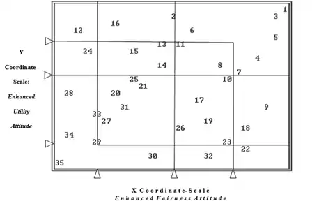
Fairness—a straight vertical line;
Utility—a straight horizontal line;
Equality—an L-shaped line;
Corrective action—an inverted-L-shaped line
The content significance of the intervals induced by these partition-lines on the X coordinate and on the Y coordinate of the POSAC space, are now identified and thereby define the contents of the X and Y Coordinate Scales of DJ attitudes.
The X-coordinate Scale, interpreted as Enhanced Fairness Attitude Scale:
- Interval 1. Low Fairness & Low Equality DJ Attitude
- Interval 2. Low Fairness & High Equality DJ Attitude
- Interval 3. High Fairness & Low Corrective Action DJ Attitude
- Interval 4. High Fairness & High Corrective Action DJ Attitude
That is, Enhanced Fairness Attitude, even if low, (interval 1 and 2) is somewhat present when Equality is favored (interval 2). And if Enhanced Fairness Attitude is high (intervals 3 and 4), it reaches the extreme level (interval 4) when Corrective Action is favored.
The Y-coordinate Scale, interpreted as Enhanced Utility Attitude Scale:
- Interval 1. Low Utility & Low Equality DJ Attitude
- Interval 2. Low Utility & High Equality DJ Attitude
- Interval 3. High Utility s & Low Corrective Action DJ Attitude
- Interval 4. High Utility & High Corrective Action DJ Attitude
That is, Enhanced Utility Attitude, even if low, (interval 1 and 2) is somewhat present when Equality is favored (interval 2). If Enhanced Utility Attitude is high (intervals 3 and 4), it reaches the extreme level (interval 4) when Corrective Action is favored. (This may well reflect the sentiment that, in the long run, the advancement of disadvantaged pupils serves the common good.)
The meanings of the fundamental variables, X and Y, while relying on the concepts of fairness and of utility, respectively, suggest new notions that modify them. The new notions were christened Enhanced (or Extended) Fairness and Enhanced (or Extended) Utility.
Complementary topics in partial order spaces
Higher order partition lines. The above simple measurement space illustrates partition-lines that are straight or have one bend. More complex measurement spaces result with items whose partition-lines have two or more bends.[27]
While partial order spaces are used mainly for analyzing score profiles (based on range facets), under certain conditions, they may be applied to the analysis of content profiles; i.e., those based on content facets.[28]
Relating POSAC Measurement Space to the SSA Concept Space. Based on the same data matrix, POSAC measurement space and Faceted SSA concept space are mathematically related. Proved relationships rely on the introduction of a new kind of coefficient, E*, the coefficient of structural similarity.[5] While E* assesses pairwise similarity between variables, it does depend on variations in the remaining n-2 variables processed. That is, in the spirit of Facet Theory, E* depends on the sampled contents as well as on the sampled population. LSA1 procedure, within 2-dimensional POSAC/LSA program, is a special version of SSA with E* as the similarity coefficient, and with lattice ("city block") as the distance function. Under specified conditions, LSA1 may be readily derived from the boundary scales of the POSAC configuration, thereby highlighting concept/measurement space duality.
Facet theory: comparisons and comments
Concerned with the entire cycle of multivariate research – concept definition, observational design, and data analysis for concept-structure and measurement, Facet Theory constitutes a novel paradigm for the behavioral sciences. Hence, only limited aspects of it can be compared with specific statistical methods.
A distinctive feature of Facet Theory is its explicit concern with the entire set of variables included in the investigated content-universe, regarding the subset of observed variables as but a sample from which inferences can be made. Hence, clusters of variables, if observed, are of no significance. They are simply unimportant artifacts of the procedure for sampling of the variables. This is in contrast with cluster analysis or factor analysis where recorded clustering patterns determine research results and interpretations. There have been various attempts to describe technical differences between Factor Analysis and Facet Theory.[29][30] Briefly, it may be said that while Factor Analysis aims to structure the set of variables selected for observation, Facet Theory aims to structure the entire content universe of all variables, observed as well as unobserved, relying on the continuity principle and using regional hypotheses as an inferential procedure.
Guttman's SSA, as well as Multidimensional Scaling (MDS) in general, were often described as a procedure for visualizing similarities (e.g., correlations) between analyzed units (e.g., variables) in which the researcher has specific interest. (See, for example, Wikipedia, October 2020: "Multidimensional scaling (MDS) is a means of visualizing the level of similarity of individual cases of a dataset"). Modern Facet Theory, however, concerned with theory construction in the behavioral sciences, assigns SSA/MDS space a different role. Regarding the analyzed units as a sample of statistical units representing all units that pertain to the content-universe, their dispersion in the SSA/MDS space is used to infer the structure of the content universe. Namely, to infer space partitionings that define components of the content-universes and their spatial interrelationships. The inferred structure, if replicated, may suggest a theory in the investigated domain and provide a basis for theory-based measurements.
Misgivings and responses
Skeptics have voiced the following reservation: Suppose you get a successful SSA map, with a partition-pattern that matches a content-classification of the mapped variables. So what? Does this map qualify as a theory?
In response, it may be pointed out that (a) consistently replicated empirical partition-patterns in a domain of research constitute a scientific lawfulness which, as such, are of interest to Science; (b) Often a partition-pattern leads to insights that explain behavior and may have potential applications. For example, the Radex Theory of Intelligence implies that inferential abilities are less differentiated by kinds of material than memory (or rule-recall, see Example 1 above). (c) Faceted SSA is a useful preliminary procedure for performing meaningful non arbitrary measurements by Multiple Scaling (POSAC). See Example 4.
A common doubt about SSA was voiced by a sympathetic but mystified user of SSA: "Smallest Space Analysis seems to come up with provocative pictures that an imaginative observer can usually make some sense of –– in fact, I have often referred to SSA as the sociologist's Rorschach test for imagination".[31] Indeed, missing in Facet Theory are statistical significance tests that would indicate the stability of discovered or hypothesized partition patterns across population samples. For example, it is not clear how to compute the probability of obtaining a hypothesized partition pattern, assuming that in fact the variables are randomly dispersed over the SSA map.
In response, facet theorists claim that in Facet Theory the stability of research results is established by replications, as is the common practice in the natural sciences. Thus, if the same partition-pattern is observed across many population samples (and if no unexplained counterexamples are recorded), confidence in the research outcome would increase. Moreover, Facet Theory adds a stringent requirement for establishing scientific lawfulness, namely that the hypothesized partition-pattern would hold also across different selections of variables, sampled from the same mapping sentence.
Facet Theory is regarded as a promising metatheory for the behavioral sciences by Clyde Coombs, an eminent psychometrician and pioneer of mathematical psychology, who commented: “It is not uncommon for a behavioral theory to be somewhat ambiguous about its domain. The result is that an experiment usually can be performed which will support it and another experiment will disconfirm it. … The problem of how to define the boundaries of a domain, especially in social and behavioral science, is subtle and complex. Guttman’s facet theory (see Shye, 1978) is, I believe, the only substantial attempt to provide a general theory for characterizing domains; in this sense, it is a metatheory. As behavioral science advances so will the need for such theory.”[32]
References
- Guttman, L. (1959). Introduction to facet design and analysis. Proceedings of the Fifteenth International Congress of Psychology, Brussels-1957. Amsterdam: North Holland, 130-132.
- Lingoes, James C. (1973). The Guttman–Lingoes nonmetric program series. Ann Arbor, Michigan: Mathesis Press.
- Guttman, Louis (1968). "A general nonmetric technique for finding the smallest coordinate space for a configuration of points". Psychometrika. 33 (4): 469–506. doi:10.1007/BF02290164. hdl:2027/uiug.30112032881820. S2CID 120611213.
- Shye, S.; Elizur, D. (1994). Introduction to Facet Theory: Content Design and Intrinsic Data Analysis in Behavioral Research. Thousand Oaks California: SAGE Publications, Inc. doi:10.4135/9781412984645. ISBN 978-0-8039-5671-1.
- Shye, Samuel (1985). Multiple Scaling: The Theory and Application of Partial Order Scalogram Analysis. Amsterdam: North-Holland. ISBN 0-444-87870-X.
- Schlesinger, I.M. (1978). On some properties of mapping sentences. In S. Shye (ed.) Theory Construction and Data Analysis in the Behavioral Sciences. San Francisco: Jossey-Bass. (A volume in honor of Louis Guttman)
- Wozner, Yochanan (1990). People Care in Institutions: A conceptual schema and its application. New York: . New York: Haworth. ISBN 1-56024-082-2.
- Veerman, (1992)., Philip E. (1992). The Rights of the Child and the Changing Image of Childhood. Dordrect, Holland: Martinus Nijhoff. ISBN 0-7923-1250-3.
- Borg, I. & Groenen, P. (2005). Modern Multidimensional Scaling: theory and applications (2nd ed.) New York: Springer-Verlag. ISBN 978-0-387-94845-4
- Kruskal, J. B. (1964). "Multidimensional scaling by optimizing goodness of fit to a nonmetric hypothesis". Psychometrika. 29: 1–27. doi:10.1007/BF02289565. S2CID 48165675 – via doi:10.1007/BF02289565.
- Borg, I & Shye, S. (1995). Facet Theory: Form and Content. Thousand Oaks CA: Sage, pp. 143–146.
- Schlesinger, I. M.; Guttman, Louis (1969). "Smallest space analysis of intelligence and achievement tests". Psychological Bulletin. 71 (2): 95–100. doi:10.1037/h0026868. ISSN 1939-1455.
- Guttman, L. (1954). A new approach to factor analysis: the radex. In P.F. Lazarsfeld (ed.) Mathemetical Thinking in the Social Sciences. New York: Free Press, 216-257.
- Shepard, R. N. (1978). The circumplex and related topological manifolds in the study of perception. In S. Shye (Ed.), Theory construction and data analysis in the behavioral sciences (pp. 29-80). San Francisco: Jossey-Bass. (A volume in honor of Louis Guttman)
- Schwartz, S.H. (1992). Universals in the Content and Structure of Values: Theoretical Advances and Empirical Tests in 20 Countries. Advances in Experimental Social Psychology. Vol. 25,1-65.
- Borg, I., Hertel, G., Krumm, S. & Bilsky, W. (2019). Work Values and Facet Theory: From Intercorrelations to Individuals. International Studies of Management & Organization, 49:3, 283-302, DOI: 10.1080/00208825.2019.1623980
- Davidson-Arad, B. (2005). Structural analyses of the quality of life of children at risk Social Indicators Research 73: 409–429.
- Canter, D. & Fritzon, K. (1998). Differentiating arsonists: A model of firesetting actions and characteristics. Legal and Criminological Psychology, 3, 73–96.
- Salfati, C. G., & Canter, D. (1999). Differentiating stranger murders: Profiling offender characteristics from behavioral styles. Behavioral Sciences and the Law, 17, 391– 406.
- Shye, Samuel (1989). "The Systemic Life Quality model: A Basis for Urban Renewal Evaluation". Social Indicators Research. 21 (4): 343–378. doi:10.1007/BF00303952. ISSN 0303-8300. JSTOR 27520775. S2CID 144914422.
- Levy, S. (1985). Lawful roles of facets in social theories. In D. Canter (Ed.) Facet Theory: Approaches to Social Research. New York: Springer.
- Laumann, Edward O.; Pappi, Franz Urban (1973). "New Directions in the Study of Community Elites". American Sociological Review. 38 (2): 212. doi:10.2307/2094396. ISSN 0003-1224. JSTOR 2094396.
- Shye, S. (2009). From the simplex of political attitudes to the radex of universal values: the development of the systemic top-down approach to value research. In Elizur, D. & Yaniv, E. (Eds.), Theory construction and multivariate analysis: applications of the Facet Approach. (11-24). Ramat-Gan, Israel: FTA Publications. ISBN 978-965-7473-01-6.
- Guttman, Louis (1944). "A Basis for Scaling Qualitative Data". American Sociological Review. 9 (2): 139–150. doi:10.2307/2086306. ISSN 0003-1224. JSTOR 2086306.
- Levinsohn, H. (1980). Radio listening and television watching among the Arab population in Israel. Jerusalem: The Israel Institute of Applied Social Research.
- Kedar, Y. & Shye, S. (2015). The measurement of distributive justice attitudes: Multiple Scaling by POSAC. Proceedings of the 15th International Facet Theory Conference, New York, August 2015 (pp. 96–105). http://fordham.bepress.com/cgi/viewcontent.cgi?article=1012&context=ftc
- Russett, B. & Shye, S. (1993). Aggressiveness, involvement and commitment in foreign policy attitudes: Multiple scaling. In Caldwell D. and McKeown T. (Eds.), Diplomacy, Force and Leadership: Essays in honor of Alexander E. George (pp. 41–60). Boulder: Westview.
- Guttman, Louis (1959). "A Structural Theory For Intergroup Beliefs and Action". American Sociological Review. 24 (3): 318–328. doi:10.2307/2089380. ISSN 0003-1224. JSTOR 2089380.
- Guttman, L. (1982). Facet Theory, Smallest Space Analysis, and Factor Analysis. Perceptual and Motor Skills, 54, 491-493. (Addendum to Guttman, R. and Shoham, I. (1982). The structure of spatial ability items: a faceted analysis. Perceptual and Motor Skills, 54, 487-493).
- Shye, S. (1988). Inductive and Deductive Reasoning: A Structural Reanalysis of Ability Tests. Journal of Applied Psychology, 73, pp. 308-311. (Appendix: Multidimensional Scaling Versus Factor Analysis: A Methodological Note).
- Marsden, P.V. & Laumann, E.O. (1978). The social structure of religious groups: a replication and methodological critique. In S. Shye (Ed.) Theory construction and data analysis in the behavioral sciences. San Francisco: Jossey-Bass. (A volume in honor of Louis Guttman).
- Coombs, C. H. (1983). Psychology and Mathematics: An Essay on Theory. Ann Arbor: University of Michigan Press 1983.
Further reading
- Guttman, R. & Greenbaum, C. W. (1998). "Facet Theory: Its Development and Current Status." European Psychologist, Vol. 3, No. 1, March 1998, pp. 13–36.
- Levy, S. (Ed.) (1994). Louis Guttman on Theory and Methodology: Selected Writings. Aldershot: Dartmouth.
- Canter (Ed.) (1985). Facet Theory: Approaches to Social Research. New York: Springer.
- Guttman, R. (1994). Radex Theory. In Robert J. Sternberg (Ed.), Encyclopedia of Human Intelligence. New York, NY: Macmillan Publishing, 907–912.