Field (geography)
In the context of spatial analysis, geographic information systems, and geographic information science, a field is a property that fills space, and varies over space, such as temperature or density.[1] This use of the term has been adopted from physics and mathematics, due to their similarity to physical fields (vector or scalar) such as the electromagnetic field or gravitational field. Synonymous terms include spatially dependent variable (geostatistics), statistical surface ( thematic mapping), and intensive property (Chemistry) and crossbreeding between these disciplines is common. The simplest formal model for a field is the function, which yields a single value given a point in space (i.e., t = f(x, y, z) )
This use of field should not be confused with that of computer science and databases, which is also frequently used in geographic information systems.
The Nature and Types of Fields
Even though the basic concept of a field came from physics, geographers have developed independent theories, data models, and analytical methods. One reason for this apparent disconnect is that although geographic fields may show patterns similar to gravity and magnetism, they can have a very different underlying nature, and be created by very different processes. Geographic fields can be classified by their ontology or fundamental nature as:
- Natural fields, properties of matter that are formed at scales below that of human perception, and thus appear continuous at human scales, such as temperature or soil moisture.
- Aggregate fields, statistically constructed properties of aggregate groups of individuals, such as Population density or tree canopy coverage.
- Fields of potential or influence, which measure conceptual, non-material quantities (and are thus most closely related to the fields of physics), such as the probability that a person at any given location will prefer to use a particular grocery store.
Geographic fields can also be categorized according to the type of domain of the measured variable, which determines the pattern of spatial change. A continuous field has a continuous (real number) domain, and typically shows gradual change over space, such as temperature or soil moisture; a discrete field, also known as a categorical coverage, has a discrete (often qualitative) domain, such as land cover type, soil class, or surface geologic formation, and typically has a pattern of regions of homogeneous value with boundaries (or transition zones) where the value changes.
Both scalar (having a single value for any location) and vector (having multiple values for any location representing different but related properties) fields are found in geographic applications, although the former is more common.
Geographic fields can exist over a temporal domain as well as space. For example, temperature varies over time as well as location in space. In fact, many of the methods used in time geography and similar spatiotemporal models treat the location of an individual as a function or field over time.
History and methods
The modeling and analysis of fields in geographic applications was developed in five essentially separate movements, which have gradually been integrated in recent years.
- Cartographic techniques for visualizing fields, including choropleth and isarithmic maps.
- The quantitative revolution of geography, starting in the 1950s, and leading to the modern discipline of spatial analysis; especially techniques such as the Gravity model.
- The development of raster GIS models and software, starting with the Canadian Geographic Information System in the 1960s, which mapped fields such as land cover type.[2]
- The technique of cartographic modeling, pioneered by Ian McHarg in the 1960s[3] and later formalized for digital implementation by Dana Tomlin as map algebra.[4]
- Geostatistics, which arose from geology starting in the 1950s.[5]
Fields are useful in geographic thought and analysis because when properties vary over space, they tend to do so in spatial patterns due to underlying spatial structures and processes. A common pattern is, according to Tobler's first law of geography: "Everything is related to everything else, but near things are more related than distant things."[6] That is, fields (especially those found in nature) tend to vary gradually, with nearby locations having similar values. This concept has been formalized as spatial dependence or spatial autocorrelation, which underlies the method of geostatistics.[7] A parallel concept that has received less publicity, but has underlain geographic theory since at least Alexander von Humboldt is spatial association, which describes how phenomena are similarly distributed.[8] This concept is regularly used in the method of map algebra.
Representation Models
Because, in theory, a field consists of an infinite number of values at an infinite number of locations, exhibiting a non-parametric pattern, only finite sample-based representations can be used in analyical and visualization tools such as GIS, statistics, and maps. Thus, several conceptual, mathematical and data models have emerged, including:
- An irregular point sample, a finite set of sample locations, at either random or strategic locations. Examples include data from weather stations or Lidar point clouds.
- A lattice, or regular point sample, consisting of locations that are evenly spaced in each cartesian direction. These are typically stored in a Raster data structure. Examples include the Digital elevation model.
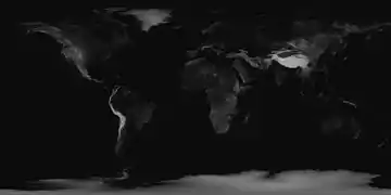 Raster DEM of Earth's surface with elevations shaded such that lighter values indicate higher elevation
 - A Choropleth, an irregular a priori partition, in which space is partitioned into regions unrelated to the field itself, such as countries, and field values are summarized over each region. These are typically stored using vector polygons. Examples would include Population density by county, derived from census returns.
- A Chorochromatic map or Area-class map, an irregular strategic partition usually used for discrete fields, in which space is partitioned into regions intended to match regions of homogeneous field value, typically stored as vector polygons. Examples include maps of geologic layers or vegetation stands.
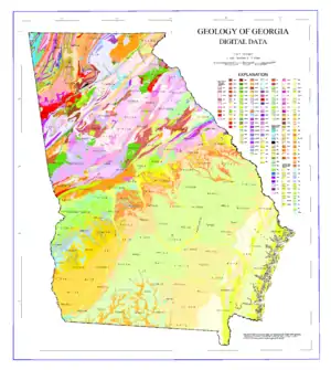 Geological map of Georgia, a chorochromatic map of the field of surface geologic formation.
 - A grid or regular partition, in which space is partitioned into equal regions (often squares), and field values are summarized over each region. These are also typically stored in a Raster data structure. Examples include the electromagnetic reflectance signature of land cover as represented in Remote sensing imagery.
- A surface, in which the field is conceptualized as a third spatial dimension, and three dimensional data models are used for representation. Examples include the Triangulated irregular network (TIN).
- An isarithm or isopleth, in which lines are drawn connecting locations of equal field value, partitioning space into regions of similar value. An example is the Contour line of elevation, commonly found on topographic maps.
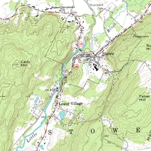 Topographic map of Stowe, Vermont. The brown contour lines represent the elevation. The contour interval is 20 feet.
The choice of representation model typically depends on a variety of factors, including the analyst's conceptual model of the phenomenon, the devices or methods available to measure the field, the tools and techniques available to analyze or visualize the field, and the models being used for other phenomena with which the field in question will be integrated. A major challenge is due to the necessity of Interpolation to estimate field values between or within the sample locations, which can lead to a number of forms of uncertainty or misinterpretation such as the Ecological fallacy and the Modifiable areal unit problem. This also means that when data is transformed from one model to another (e.g., generating a DEM from a Lidar point cloud), the result will be less certain than the source.
See also
- Feature (geography)
References
- Peuquet, Donna J., Barry Smith, Berit Brogaard, ed. The Ontology of Fields, Report of a Specialist Meeting Held under the Auspices of the Varenius Project, June 11-13, 1998, 1999
- Fisher, Terry & Connie MacDonald, An Overview of the Canada Geographic Information System (CGIS), Proceedings of Auto-Carto IV, Cartography and Geographic Information Society, 1979
- McHarg, Ian, Design with Nature, American Museum of Natural History, 1969
- Tomlin, C. Dana, Geographic information systems and cartographic modelling Prentice-Hall 1990.
- Griffith, Daniel A., Spatial Statistics: A quantitative geographer's perspective, Spatial Statistics, 1:3-15, DOI: 10.1016/j.spasta.2012.03.005
- Tobler W., (1970) "A computer movie simulating urban growth in the Detroit region". Economic Geography, 46(Supplement): 234–240.
- Cliff, A. and J. Ord, Spatial Autocorrelation, Pion, 1973
- Bradley Miller Fundamentals of Spatial Prediction www.geographer-miller.com, 2014.