Langevin equation
In physics, a Langevin equation (named after Paul Langevin) is a stochastic differential equation describing the time evolution of a subset of the degrees of freedom. These degrees of freedom typically are collective (macroscopic) variables changing only slowly in comparison to the other (microscopic) variables of the system. The fast (microscopic) variables are responsible for the stochastic nature of the Langevin equation. One application is to Brownian motion, calculating the statistics of the random motion of a small particle in a fluid due to collisions with the surrounding molecules in thermal motion.
Brownian motion as a prototype
The original Langevin equation[1] describes Brownian motion, the apparently random movement of a particle in a fluid due to collisions with the molecules of the fluid,

The degrees of freedom of interest here is the velocity of the particle, denotes the particle's mass. The force acting on the particle is written as a sum of a viscous force proportional to the particle's velocity (Stokes' law), and a noise term (the name given in physical contexts to terms in stochastic differential equations which are stochastic processes) representing the effect of the collisions with the molecules of the fluid. The force has a Gaussian probability distribution with correlation function


where is Boltzmann's constant, is the temperature and is the i-th component of the vector . The -function form of the correlations in time means that the force at a time is assumed to be completely uncorrelated with the force at any other time. This is an approximation; the actual random force has a nonzero correlation time corresponding to the collision time of the molecules. However, the Langevin equation is used to describe the motion of a "macroscopic" particle at a much longer time scale, and in this limit the -correlation and the Langevin equation becomes virtually exact.


Another prototypical feature of the Langevin equation is the occurrence of the damping coefficient in the correlation function of the random force, a fact also known as Einstein relation.

Mathematical aspects
A strictly -correlated fluctuating force is not a function in the usual mathematical sense and even the derivative is not defined in this limit. This problem disappears when the Langevin equation is written in integral form and a Langevin equation always should be interpreted as an abbreviation for its time integral. The general mathematical term for equations of this type is "stochastic differential equation".


Another mathematical ambiguity occurs for (rather special) Langevin equations with a multiplicative noise, that is terms like on the r.h.s.. Such equations can be interpreted according to Stratonovich- or Ito- scheme, and if the derivation of the Langevin equation does not tell which one to use it is questionable anyhow. See Itō calculus.[2]

Generic Langevin equation
There is a formal derivation of a generic Langevin equation from classical mechanics.[3][4] This generic equation plays a central role in the theory of critical dynamics,[5] and other areas of nonequilibrium statistical mechanics. The equation for Brownian motion above is a special case.
An essential condition of the derivation is a criterion dividing the degrees of freedom into the categories slow and fast. For example, local thermodynamic equilibrium in a liquid is reached within a few collision times. But it takes much longer for densities of conserved quantities like mass and energy to relax to equilibrium. Densities of conserved quantities, and in particular their long wavelength components, thus are slow variable candidates. Technically this division is realized with the Zwanzig projection operator,[6] the essential tool in the derivation. The derivation is not completely rigorous because it relies on (plausible) assumptions akin to assumptions required elsewhere in basic statistical mechanics.
Let denote the slow variables. The generic Langevin equation then reads


The fluctuating force obeys a Gaussian probability distribution with correlation function

This implies the Onsager reciprocity relation for the damping coefficients . The dependence of on is negligible in most cases. The symbol denotes the Hamiltonian of the system, where is the equilibrium probability distribution of the variables . Finally, is the projection of the Poisson bracket of the slow variables and onto the space of slow variables.


In the Brownian motion case one would have , or and . The equation of motion for is exact, there is no fluctuating force and no damping coefficient .


Examples
Trajectories of free Brownian particles
Consider a free particle of mass with equation of motion described by

where is the particle velocity, is the particle mobility, and is a rapidly fluctuating force whose time-average vanishes over a characteristic timescale of particle collisions, i.e. . The general solution to the equation of motion is


where is the relaxation time of the Brownian motion. As expected from the random nature of Brownian motion, the average drift velocity quickly decays to zero at . It can also be shown that the autocorrelation function of the particle velocity is given by[7]


where we have used the property that the variables and become uncorrelated for time separations . Besides, the value of is set to be equal to such that it obeys the equipartition theorem. Note that if the system is initially at thermal equilibrium already with , then for all , meaning that the system remains at equilibrium at all times.


The velocity of the Brownian particle can be integrated to yield its trajectory (assuming it is initially at the origin)


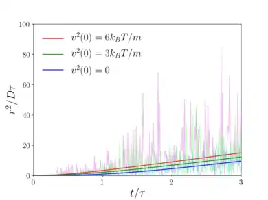
Hence, the resultant average displacement asymptotes to as the system relaxes and randomness takes over. In addition, the mean squared displacement can be determined similarly to the preceding calculation to be


It can be seen that , indicating that the motion of Brownian particles at timescales much shorter than the relaxation time of the system is (approximately) time-reversal invariant. On the other hand, , which suggests that the long-term random motion of Brownian particles is an irreversible dissipative process. Here we have made use of the Einstein–Smoluchowski relation , where is the diffusion coefficient of the fluid.


Harmonic oscillator in a fluid

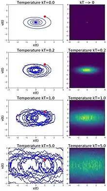
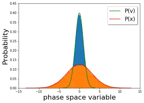
A particle in a fluid is also described by the Langevin equation with a potential, a damping force and thermal fluctuations given by the fluctuation dissipation theorem. If the potential is a harmonic oscillator potential then the constant energy curves are ellipses as shown in Figure 1 below. However, in the presence of a dissipation force a particle keeps losing energy to the environment. On the other hand, the thermal fluctuation randomly adds energy to the particle. In the absence of the thermal fluctuations the particle continuously loses kinetic energy and the phase portrait of the time evolution of the velocity vs. position looks like an ellipse that is spiraling in until it reaches zero velocity. Conversely, the thermal fluctuations provide kicks to the particles that do not allow the particle to lose all its energy. So, at long times, the initial ensemble of stochastic oscillators to spread out, eventually reaching thermal equilibrium, for whom the distribution of velocity and position is given by the Maxwell–Boltzmann distribution. In the plot below (Figure 2), the long time velocity distribution (orange) and position distributions (blue) in a harmonic potential ( ) is plotted with the Boltzmann probabilities for velocity (red) and position (green). We see that the late time behavior depicts thermal equilibrium.

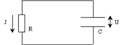
Thermal noise in an electrical resistor
There is a close analogy between the paradigmatic Brownian particle discussed above and Johnson noise, the electric voltage generated by thermal fluctuations in every resistor.[8] The diagram at the right shows an electric circuit consisting of a resistance R and a capacitance C. The slow variable is the voltage U between the ends of the resistor. The Hamiltonian reads , and the Langevin equation becomes


This equation may be used to determine the correlation function

which becomes a white noise (Johnson noise) when the capacitance C becomes negligibly small.
Critical dynamics
The dynamics of the order parameter of a second order phase transition slows down near the critical point and can be described with a Langevin equation.[5] The simplest case is the universality class "model A" with a non-conserved scalar order parameter, realized for instance in axial ferromagnets,


Other universality classes (the nomenclature is "model A",..., "model J") contain a diffusing order parameter, order parameters with several components, other critical variables and/or contributions from Poisson brackets.[5]
Recovering Boltzmann statistics
Langevin equations must reproduce the Boltzmann distribution. 1-dimensional overdamped Brownian motion is an instructive example. The overdamped case is realized when the inertia of the particle is negligible in comparison to the damping force. The trajectory of the particle in a potential is described by the Langevin equation


where the noise is characterized by and is the damping constant. We would like to compute the distribution of the particle's position in the course of time. A direct way to determine this distribution is to introduce a test function , and to look at the average of this function over all realizations (ensemble average)


If remains finite then this quantity is null. Moreover, using the Stratonovich interpretation, we are able to get rid of the eta in the second term so that we end up with

where we make use of the probability density function . This is done by explicitly computing the average,

where the second term was integrated by parts (hence the negative sign). Since this is true for arbitrary functions , we must have:

thus recovering the Boltzmann distribution

Equivalent techniques
A solution of a Langevin equation for a particular realization of the fluctuating force is of no interest by itself; what is of interest are correlation functions of the slow variables after averaging over the fluctuating force. Such correlation functions also may be determined with other (equivalent) techniques.
Fokker–Planck equation
A Fokker–Planck equation is a deterministic equation for the time dependent probability density of stochastic variables . The Fokker–Planck equation corresponding to the generic Langevin equation above may be derived with standard techniques (see for instance ref.[9]),


The equilibrium distribution is a stationary solution.

Path integral
A path integral equivalent to a Langevin equation may be obtained from the corresponding Fokker–Planck equation or by transforming the Gaussian probability distribution of the fluctuating force to a probability distribution of the slow variables, schematically . The functional determinant and associated mathematical subtleties drop out if the Langevin equation is discretized in the natural (causal) way, where depends on but not on . It turns out to be convenient to introduce auxiliary response variables . The path integral equivalent to the generic Langevin equation then reads [10]


where is a normalization factor and


The path integral formulation doesn't add anything new, but it does allow for the use of tools from quantum field theory; for example perturbation and renormalization group methods (if these make sense).
See also
References
- Langevin, P. (1908). "Sur la théorie du mouvement brownien [On the Theory of Brownian Motion]". C. R. Acad. Sci. Paris. 146: 530–533.; reviewed by D. S. Lemons & A. Gythiel: Paul Langevin’s 1908 paper "On the Theory of Brownian Motion" [...], Am. J. Phys. 65, 1079 (1997), doi:10.1119/1.18725
- Stochastic Processes in Physics and Chemistry. Elsevier. 2007. doi:10.1016/b978-0-444-52965-7.x5000-4. ISBN 978-0-444-52965-7.
- Kawasaki, K. (1973). "Simple derivations of generalized linear and nonlinear Langevin equations". J. Phys. A: Math. Nucl. Gen. 6 (9): 1289–1295. Bibcode:1973JPhA....6.1289K. doi:10.1088/0305-4470/6/9/004.
- Dengler, R. (2015). "Another derivation of generalized Langevin equations". arXiv:1506.02650v2 [physics.class-ph].
- Hohenberg, P. C.; Halperin, B. I. (1977). "Theory of dynamic critical phenomena". Reviews of Modern Physics. 49 (3): 435–479. Bibcode:1977RvMP...49..435H. doi:10.1103/RevModPhys.49.435.
- Zwanzig, R. (1961). "Memory effects in irreversible thermodynamics". Phys. Rev. 124 (4): 983–992. Bibcode:1961PhRv..124..983Z. doi:10.1103/PhysRev.124.983.
- Pathria RK (1972). Statistical Mechanics. Oxford: Pergamon Press. pp. 443, 474–477. ISBN 0-08-018994-6.
- Johnson, J. (1928). "Thermal Agitation of Electricity in Conductors". Phys. Rev. 32 (1): 97. Bibcode:1928PhRv...32...97J. doi:10.1103/PhysRev.32.97.
- Ichimaru, S. (1973), Basic Principles of Plasma Physics (1st. ed.), USA: Benjamin, p. 231, ISBN 0805387536
- Janssen, H. K. (1976). "Lagrangean for Classical Field Dynamics and Renormalization Group Calculations of Dynamical Critical Properties". Z. Phys. B. 23 (4): 377–380. Bibcode:1976ZPhyB..23..377J. doi:10.1007/BF01316547. S2CID 121216943.
Further reading
- W. T. Coffey (Trinity College, Dublin, Ireland) and Yu P. Kalmykov (Université de Perpignan, France, The Langevin Equation: With Applications to Stochastic Problems in Physics, Chemistry and Electrical Engineering (Third edition), World Scientific Series in Contemporary Chemical Physics - Vol 27.
- Reif, F. Fundamentals of Statistical and Thermal Physics, McGraw Hill New York, 1965. See section 15.5 Langevin Equation
- R. Friedrich, J. Peinke and Ch. Renner. How to Quantify Deterministic and Random Influences on the Statistics of the Foreign Exchange Market, Phys. Rev. Lett. 84, 5224 - 5227 (2000)
- L.C.G. Rogers and D. Williams. Diffusions, Markov Processes, and Martingales, Cambridge Mathematical Library, Cambridge University Press, Cambridge, reprint of 2nd (1994) edition, 2000.