Radial basis function interpolation

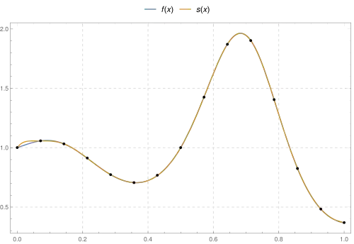
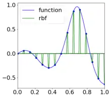
Let ${\displaystyle f(x)=\exp(x\cos(3\pi x))}$ and let ${\displaystyle x_{k}={\frac {k}{14}},k=0,1,\dots ,14}$ be 15 equally spaced points on the interval ${\displaystyle [0,1]}$. We will form ${\displaystyle s(x)=\sum \limits _{k=0}^{14}w_{k}\varphi (\|x-x_{k}\|)}$ where ${\displaystyle \varphi }$ is a radial basis function, and choose ${\displaystyle w_{k},k=0,1,\dots ,14}$ such that ${\displaystyle s(x_{k})=f(x_{k}),k=0,1,\dots ,14}$ (${\displaystyle s}$ interpolates ${\displaystyle f}$ at the chosen points). In matrix notation this can be written as

$${\displaystyle {\begin{bmatrix}\varphi (\|x_{0}-x_{0}\|)&\varphi (\|x_{1}-x_{0}\|)&\dots &\varphi (\|x_{14}-x_{0}\|)\\\varphi (\|x_{0}-x_{1}\|)&\varphi (\|x_{1}-x_{1}\|)&\dots &\varphi (\|x_{14}-x_{1}\|)\\\vdots &\vdots &\ddots &\vdots \\\varphi (\|x_{0}-x_{14}\|)&\varphi (\|x_{1}-x_{14}\|)&\dots &\varphi (\|x_{14}-x_{14}\|)\\\end{bmatrix}}{\begin{bmatrix}w_{0}\\w_{1}\\\vdots \\w_{14}\end{bmatrix}}={\begin{bmatrix}f(x_{0})\\f(x_{1})\\\vdots \\f(x_{14})\end{bmatrix}}.}$$

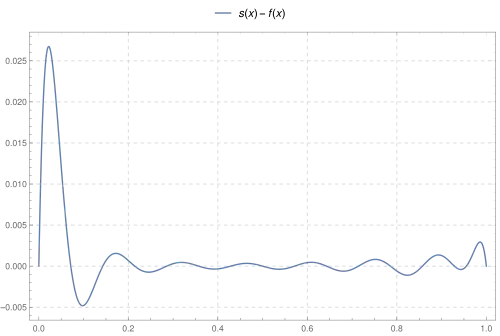
Choosing ${\displaystyle \varphi (r)=\exp(-(\varepsilon r)^{2})}$, the Gaussian, with a shape parameter of ${\displaystyle \varepsilon =3}$, we can then solve the matrix equation for the weights and plot the interpolant. Plotting the interpolating function below, we see that it is visually the same everywhere except near the left boundary (an example of Runge's phenomenon), where it is still a very close approximation. More precisely the maximum error is roughly ${\displaystyle \|f-s\|_{\infty }\approx 0.0267414}$ at ${\displaystyle x=0.0220012}$.

The function ${\displaystyle f(x)=\exp(x\cos(3\pi x))}$ sampled at 15 uniform nodes between 0 and 1, interpolated using the Gaussian RBF with a shape parameter of ${\displaystyle \varepsilon =3}$.

The interpolation error, ${\displaystyle s(x)-f(x)}$, for the plot to the left.

The Mairhuber–Curtis theorem says that for any open set ${\displaystyle V}$ in ${\displaystyle \mathbb {R} ^{n}}$ with ${\displaystyle n\geq 2}$, and ${\displaystyle f_{1},f_{2},\dots ,f_{n}}$ linearly independent functions on ${\displaystyle V}$, there exists a set of ${\displaystyle n}$ points in the domain such that the interpolation matrix

$${\displaystyle {\begin{bmatrix}f_{1}(x_{1})&f_{2}(x_{1})&\dots &f_{n}(x_{1})\\f_{1}(x_{2})&f_{2}(x_{2})&\dots &f_{n}(x_{2})\\\vdots &\vdots &\ddots &\vdots \\f_{1}(x_{n})&f_{2}(x_{n})&\dots &f_{n}(x_{n})\end{bmatrix}}}$$

is singular.[5]

This means that if one wishes to have a general interpolation algorithm, one must choose the basis functions to depend on the interpolation points. In 1971, Rolland Hardy developed a method of interpolating scattered data using interpolants of the form ${\displaystyle s(\mathbf {x} )=\sum \limits _{k=1}^{N}{\sqrt {\|\mathbf {x} -\mathbf {x} _{k}\|^{2}+C}}}$. This is interpolation using a basis of shifted multiquadric functions, now more commonly written as ${\displaystyle \varphi (r)={\sqrt {1+(\varepsilon r)^{2}}}}$, and is the first instance of radial basis function interpolation.[6] It has been shown that the resulting interpolation matrix will always be non-singular. This does not violate the Mairhuber–Curtis theorem since the basis functions depend on the points of interpolation. Choosing a radial kernel such that the interpolation matrix is non-singular is exactly the definition of a radial basis function. It has been shown that any function that is completely monotone will have this property, including the Gaussian, inverse quadratic, and inverse multiquadric functions.[7]

Many radial basis functions have a parameter that controls their relative flatness or peakedness. This parameter is usually represented by the symbol ${\displaystyle \varepsilon }$ with the function becoming increasingly flat as ${\displaystyle \varepsilon \to 0}$. For example, Rolland Hardy used the formula ${\displaystyle \varphi (r)={\sqrt {r^{2}+C}}}$ for the multiquadric, however nowadays the formula ${\displaystyle \varphi (r)={\sqrt {1+(\varepsilon r)^{2}}}}$ is used instead. These formulas are equivalent up to a scale factor. This factor is inconsequential since the basis vectors have the same span and the interpolation weights will compensate. By convention, the basis function is scaled such that ${\displaystyle \varphi (0)=1}$ as seen in the plots of the Gaussian functions and the bump functions.

• 
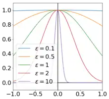  A Gaussian function for several choices of ${\displaystyle \varepsilon }$
• 
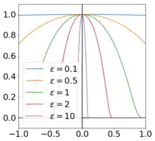  A plot of the scaled bump function with several choices of shape parameter

An RBF interpolant of the function f(x)=e^(x*cos(3*pi*x))-1 sampled at 15 points, using Gaussians, with a very large shape parameter e=100. The "bed-of-nails interpolant."

A consequence of this choice, is that the interpolation matrix approaches the identity matrix as ${\displaystyle \varepsilon \to \infty }$ leading to stability when solving the matrix system. The resulting interpolant will in general be a poor approximation to the function since it will be near zero everywhere, except near the interpolation points where it will sharply peak – the so-called "bed-of-nails interpolant" (as seen in the plot to the right).

A plot of the condition number by the shape parameter for a 15x15 radial basis function interpolation matrix using the Gaussian

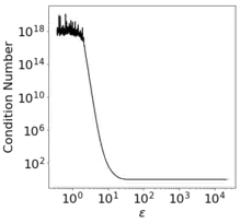
On the opposite side of the spectrum, the condition number of the interpolation matrix will diverge to infinity as ${\displaystyle \varepsilon \to 0}$ leading to ill-conditioning of the system. In practice, one chooses a shape parameter so that the interpolation matrix is "on the edge of ill-conditioning" (eg. with a condition number of roughly ${\displaystyle 10^{12}}$ for double-precision floating point).

There are sometimes other factors to consider when choosing a shape-parameter. For example the bump function

$${\displaystyle \varphi (r)={\begin{cases}\exp \left(-{\frac {1}{1-(\varepsilon r)^{2}}}\right)&{\mbox{ for }}r<{\frac {1}{\varepsilon }}\\0&{\mbox{ otherwise}}\end{cases}}}$$

has a compact support (it is zero everywhere except when ${\displaystyle r<{\tfrac {1}{\varepsilon }}}$) leading to a sparse interpolation matrix.

Some radial basis functions such as the polyharmonic splines have no shape-parameter.

References

- Buhmann, Martin; Nira, Dyn (June 1993). "Spectral convergence of multiquadric interpolation". Proceedings of the Edinburgh Mathematical Society. 36 (2): 319–333. doi:10.1017/S0013091500018411.
- Flyer, Natasha; Barnett, Gregory A.; Wicker, Louis J. (2016). "Enhancing finite differences with radial basis functions: Experiments on the Navier–Stokes equations". Journal of Computational Physics. 316: 39–62. doi:10.1016/j.jcp.2016.02.078.
- Wong, S.M.; Hon, Y.C.; Golberg, M.A. (2002). "Compactly supported radial basis functions for shallow water equations". Applied Mathematics and Computation. 127 (1): 79–101. doi:10.1016/S0096-3003(01)00006-6.
- Flyer, Natasha; Wright, Grady B. (2009). "A radial basis function method for the shallow water equations on a sphere". Proceedings of the Royal Society A: Mathematical, Physical and Engineering Sciences. 465 (2106): 1949–1976. doi:10.1098/rspa.2009.0033.
- Mairhuber, John C. (1956). "On Haar's Theorem Concerning Chebychev Approximation Problems Having Unique Solutions". Proceedings of the American Mathematical Society. 7 (4): 609–615. JSTOR 2033359.
- Hardy, Rolland L. (1971). "Multiquadric equations of topography and other irregular surfaces". Journal of Geophysical Research. 7 (8): 1905–1915. doi:10.1029/JB076i008p01905.
- Fasshaur, Greg (2007). Meshfree Approximation Methods with MATLAB. World Scientific Publishing. ISBN 978-981-270-633-1.