Tutte polynomial
The Tutte polynomial, also called the dichromate or the Tutte–Whitney polynomial, is a graph polynomial. It is a polynomial in two variables which plays an important role in graph theory. It is defined for every undirected graph and contains information about how the graph is connected. It is denoted by .
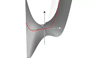
The importance of this polynomial stems from the information it contains about . Though originally studied in algebraic graph theory as a generalization of counting problems related to graph coloring and nowhere-zero flow, it contains several famous other specializations from other sciences such as the Jones polynomial from knot theory and the partition functions of the Potts model from statistical physics. It is also the source of several central computational problems in theoretical computer science.
The Tutte polynomial has several equivalent definitions. It is equivalent to Whitney’s rank polynomial, Tutte’s own dichromatic polynomial and Fortuin–Kasteleyn’s random cluster model under simple transformations. It is essentially a generating function for the number of edge sets of a given size and connected components, with immediate generalizations to matroids. It is also the most general graph invariant that can be defined by a deletion–contraction recurrence. Several textbooks about graph theory and matroid theory devote entire chapters to it.[1][2][3]
Definitions
Definition. For an undirected graph one may define the Tutte polynomial as
where denotes the number of connected components of the graph . In this definition it is clear that is well-defined and a polynomial in and .
The same definition can be given using slightly different notation by letting denote the rank of the graph . Then the Whitney rank generating function is defined as
The two functions are equivalent under a simple change of variables:
Tutte’s dichromatic polynomial is the result of another simple transformation:
Tutte’s original definition of is equivalent but less easily stated. For connected we set
where denotes the number of spanning trees of internal activity and external activity .
A third definition uses a deletion–contraction recurrence. The edge contraction of graph is the graph obtained by merging the vertices and and removing the edge . We write for the graph where the edge is merely removed. Then the Tutte polynomial is defined by the recurrence relation
if is neither a loop nor a bridge, with base case
if contains bridges and loops and no other edges. Especially, if contains no edges.
The random cluster model from statistical mechanics due to Fortuin & Kasteleyn (1972) provides yet another equivalent definition.[4] The partition sum
is equivalent to under the transformation[5]
Properties
The Tutte polynomial factors into connected components. If is the union of disjoint graphs and then
If is planar and denotes its dual graph then
Especially, the chromatic polynomial of a planar graph is the flow polynomial of its dual. Tutte refers to such functions as V-functions.[6]
Examples
Isomorphic graphs have the same Tutte polynomial, but the converse is not true. For example, the Tutte polynomial of every tree on edges is .
Tutte polynomials are often given in tabular form by listing the coefficients of in row and column . For example, the Tutte polynomial of the Petersen graph,
is given by the following table.
| 0 | 36 | 84 | 75 | 35 | 9 | 1 |
| 36 | 168 | 171 | 65 | 10 | ||
| 120 | 240 | 105 | 15 | |||
| 180 | 170 | 30 | ||||
| 170 | 70 | |||||
| 114 | 12 | |||||
| 56 | ||||||
| 21 | ||||||
| 6 | ||||||
| 1 |
Other example, the Tutte polynomial of the octahedron graph is given by
History
W. T. Tutte’s interest in the deletion–contraction formula started in his undergraduate days at Trinity College, Cambridge, originally motivated by perfect rectangles and spanning trees. He often applied the formula in his research and “wondered if there were other interesting functions of graphs, invariant under isomorphism, with similar recursion formulae.”[6] R. M. Foster had already observed that the chromatic polynomial is one such function, and Tutte began to discover more. His original terminology for graph invariants that satisfy the deletion–contraction recursion was W-function, and V-function if multiplicative over components. Tutte writes, “Playing with my W-functions I obtained a two-variable polynomial from which either the chromatic polynomial or the flow-polynomial could be obtained by setting one of the variables equal to zero, and adjusting signs.”[6] Tutte called this function the dichromate, as he saw it as a generalization of the chromatic polynomial to two variables, but it is usually referred to as the Tutte polynomial. In Tutte’s words, “This may be unfair to Hassler Whitney who knew and used analogous coefficients without bothering to affix them to two variables.” (There is “notable confusion”[7] about the terms dichromate and dichromatic polynomial, introduced by Tutte in different paper, and which differ only slightly.) The generalisation of the Tutte polynomial to matroids was first published by Crapo, though it appears already in Tutte’s thesis.[8]
Independently of the work in algebraic graph theory, Potts began studying the partition function of certain models in statistical mechanics in 1952. The work by Fortuin and Kasteleyn[9] on the random cluster model, a generalisation of the Potts model, provided a unifying expression that showed the relation to the Tutte polynomial.[8]
Specialisations
At various points and lines of the -plane, the Tutte polynomial evaluates to quantities that have been studied in their own right in diverse fields of mathematics and physics. Part of the appeal of the Tutte polynomial comes from the unifying framework it provides for analysing these quantities.
Chromatic polynomial
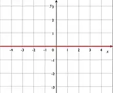
At , the Tutte polynomial specialises to the chromatic polynomial,
where denotes the number of connected components of G.
For integer λ the value of chromatic polynomial equals the number of vertex colourings of G using a set of λ colours. It is clear that does not depend on the set of colours. What is less clear is that it is the evaluation at λ of a polynomial with integer coefficients. To see this, we observe:
- If G has n vertices and no edges, then .
- If G contains a loop (a single edge connecting a vertex to itself), then .
- If e is an edge which is not a loop, then
The three conditions above enable us to calculate , by applying a sequence of edge deletions and contractions; but they give no guarantee that a different sequence of deletions and contractions will lead to the same value. The guarantee comes from the fact that counts something, independently of the recurrence. In particular,
gives the number of acyclic orientations.
Jones polynomial
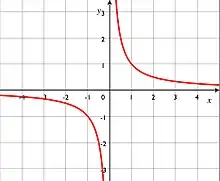
Along the hyperbola , the Tutte polynomial of a planar graph specialises to the Jones polynomial of an associated alternating knot.
(2,1)
counts the number of forests, i.e., the number of acyclic edge subsets.
(1,1)
counts the number of spanning forests (edge subsets without cycles and the same number of connected components as G). If the graph is connected, counts the number of spanning trees.
(1,2)
counts the number of spanning subgraphs (edge subsets with the same number of connected components as G).
(2,0)
counts the number of acyclic orientations of G.[10]
(0,2)
counts the number of strongly connected orientations of G.[11]
(2,2)
is the number where is the number of edges of graph G.
(0,−2)
If G is a 4-regular graph, then
counts the number of Eulerian orientations of G. Here is the number of connected components of G.[10]
(3,3)
If G is the m × n grid graph, then counts the number of ways to tile a rectangle of width 4m and height 4n with T-tetrominoes.[12][13]
If G is a planar graph, then equals the sum over weighted Eulerian orientations in a medial graph of G, where the weight of an orientation is 2 to the number of saddle vertices of the orientation (that is, the number of vertices with incident edges cyclicly ordered "in, out, in out").[14]
Potts and Ising models
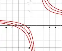
Define the hyperbola in the xy−plane:
the Tutte polynomial specialises to the partition function, of the Ising model studied in statistical physics. Specifically, along the hyperbola the two are related by the equation:[15]
In particular,
for all complex α.
More generally, if for any positive integer q, we define the hyperbola:
then the Tutte polynomial specialises to the partition function of the q-state Potts model. Various physical quantities analysed in the framework of the Potts model translate to specific parts of the .
| Potts model | Tutte polynomial |
|---|---|
| Ferromagnetic | Positive branch of |
| Antiferromagnetic | Negative branch of with |
| High temperature | Asymptote of to |
| Low temperature ferromagnetic | Positive branch of asymptotic to |
| Zero temperature antiferromagnetic | Graph q-colouring, i.e., |
Flow polynomial
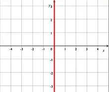
At , the Tutte polynomial specialises to the flow polynomial studied in combinatorics. For a connected and undirected graph G and integer k, a nowhere-zero k-flow is an assignment of “flow” values to the edges of an arbitrary orientation of G such that the total flow entering and leaving each vertex is congruent modulo k. The flow polynomial denotes the number of nowhere-zero k-flows. This value is intimately connected with the chromatic polynomial, in fact, if G is a planar graph, the chromatic polynomial of G is equivalent to the flow polynomial of its dual graph in the sense that
Theorem (Tutte).
The connection to the Tutte polynomial is given by:
Reliability polynomial
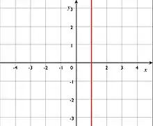
At , the Tutte polynomial specialises to the all-terminal reliability polynomial studied in network theory. For a connected graph G remove every edge with probability p; this models a network subject to random edge failures. Then the reliability polynomial is a function , a polynomial in p, that gives the probability that every pair of vertices in G remains connected after the edges fail. The connection to the Tutte polynomial is given by
Dichromatic polynomial
Tutte also defined a closer 2-variable generalization of the chromatic polynomial, the dichromatic polynomial of a graph. This is
where is the number of connected components of the spanning subgraph (V,A). This is related to the corank-nullity polynomial by
The dichromatic polynomial does not generalize to matroids because k(A) is not a matroid property: different graphs with the same matroid can have different numbers of connected components.
Related polynomials
Martin polynomial
The Martin polynomial of an oriented 4-regular graph was defined by Pierre Martin in 1977.[17] He showed that if G is a plane graph and is its directed medial graph, then
Algorithms
Deletion–contraction
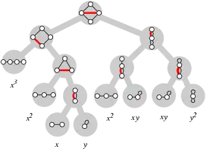
The deletion–contraction recurrence for the Tutte polynomial,
immediately yields a recursive algorithm for computing it for a given graph: as long as you can find an edge e that is not a loop or bridge, recursively compute the Tutte polynomial for when that edge is deleted, and when that edge is contracted. Then add the two sub-results together to get the overall Tutte polynomial for the graph.
The base case is a monomial where m is the number of bridges, and n is the number of loops.
Within a polynomial factor, the running time t of this algorithm can be expressed in terms of the number of vertices n and the number of edges m of the graph,
a recurrence relation that scales as the Fibonacci numbers with solution[18]
The analysis can be improved to within a polynomial factor of the number of spanning trees of the input graph.[19] For sparse graphs with this running time is . For regular graphs of degree k, the number of spanning trees can be bounded by
where
so the deletion–contraction algorithm runs within a polynomial factor of this bound. For example:[20]
In practice, graph isomorphism testing is used to avoid some recursive calls. This approach works well for graphs that are quite sparse and exhibit many symmetries; the performance of the algorithm depends on the heuristic used to pick the edge e.[19][21][22]
Gaussian elimination
In some restricted instances, the Tutte polynomial can be computed in polynomial time, ultimately because Gaussian elimination efficiently computes the matrix operations determinant and Pfaffian. These algorithms are themselves important results from algebraic graph theory and statistical mechanics.
equals the number of spanning trees of a connected graph. This is computable in polynomial time as the determinant of a maximal principal submatrix of the Laplacian matrix of G, an early result in algebraic graph theory known as Kirchhoff’s Matrix–Tree theorem. Likewise, the dimension of the bicycle space at can be computed in polynomial time by Gaussian elimination.
For planar graphs, the partition function of the Ising model, i.e., the Tutte polynomial at the hyperbola , can be expressed as a Pfaffian and computed efficiently via the FKT algorithm. This idea was developed by Fisher, Kasteleyn, and Temperley to compute the number of dimer covers of a planar lattice model.
Markov chain Monte Carlo
Using a Markov chain Monte Carlo method, the Tutte polynomial can be arbitrarily well approximated along the positive branch of , equivalently, the partition function of the ferromagnetic Ising model. This exploits the close connection between the Ising model and the problem of counting matchings in a graph. The idea behind this celebrated result of Jerrum and Sinclair[23] is to set up a Markov chain whose states are the matchings of the input graph. The transitions are defined by choosing edges at random and modifying the matching accordingly. The resulting Markov chain is rapidly mixing and leads to “sufficiently random” matchings, which can be used to recover the partition function using random sampling. The resulting algorithm is a fully polynomial-time randomized approximation scheme (fpras).
Computational complexity
Several computational problems are associated with the Tutte polynomial. The most straightforward one is
- Input: A graph
- Output: The coefficients of
In particular, the output allows evaluating which is equivalent to counting the number of 3-colourings of G. This latter question is #P-complete, even when restricted to the family of planar graphs, so the problem of computing the coefficients of the Tutte polynomial for a given graph is #P-hard even for planar graphs.
Much more attention has been given to the family of problems called Tutte defined for every complex pair :
- Input: A graph
- Output: The value of
The hardness of these problems varies with the coordinates .
Exact computation
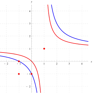
If both x and y are non-negative integers, the problem belongs to #P. For general integer pairs, the Tutte polynomial contains negative terms, which places the problem in the complexity class GapP, the closure of #P under subtraction. To accommodate rational coordinates , one can define a rational analogue of #P.[24]
The computational complexity of exactly computing falls into one of two classes for any . The problem is #P-hard unless lies on the hyperbola or is one of the points
in which cases it is computable in polynomial time.[25] If the problem is restricted to the class of planar graphs, the points on the hyperbola become polynomial-time computable as well. All other points remain #P-hard, even for bipartite planar graphs.[26] In his paper on the dichotomy for planar graphs, Vertigan claims (in his conclusion) that the same result holds when further restricted to graphs with vertex degree at most three, save for the point , which counts nowhere-zero Z3-flows and is computable in polynomial time.[27]
These results contain several notable special cases. For example, the problem of computing the partition function of the Ising model is #P-hard in general, even though celebrated algorithms of Onsager and Fisher solve it for planar lattices. Also, the Jones polynomial is #P-hard to compute. Finally, computing the number of four-colorings of a planar graph is #P-complete, even though the decision problem is trivial by the four color theorem. In contrast, it is easy to see that counting the number of three-colorings for planar graphs is #P-complete because the decision problem is known to be NP-complete via a parsimonious reduction.
Approximation
The question which points admit a good approximation algorithm has been very well studied. Apart from the points that can be computed exactly in polynomial time, the only approximation algorithm known for is Jerrum and Sinclair’s FPRAS, which works for points on the “Ising” hyperbola for y > 0. If the input graphs are restricted to dense instances, with degree , there is an FPRAS if x ≥ 1, y ≥ 1.[28]
Even though the situation is not as well understood as for exact computation, large areas of the plane are known to be hard to approximate.[24]
See also
- Bollobás–Riordan polynomial
- A Tutte–Grothendieck invariant is any evaluation of the Tutte polynomial
Notes
- Bollobás 1998, chapter 10.
- Biggs 1993, chapter 13.
- Godsil & Royle 2004, chap. 15.
- Sokal 2005.
- Sokal 2005, eq. (2.26).
- Tutte 2004.
- Welsh.
- Farr 2007.
- Fortuin & Kasteleyn 1972.
- Welsh 1999.
- Las Vergnas 1980.
- Korn & Pak 2004.
- See Korn & Pak 2003 for combinatorial interpretations of many other points.
- Las Vergnas 1988.
- Welsh 1993, p. 62.
- Welsh & Merino 2000.
- Martin 1977.
- Wilf 1986, p. 46.
- Sekine, Imai & Tani 1995.
- Chung & Yau 1999, following Björklund et al. 2008.
- Haggard, Pearce & Royle 2010.
- Pearce, Haggard & Royle 2010.
- Jerrum & Sinclair 1993.
- Goldberg & Jerrum 2008.
- Jaeger, Vertigan & Welsh 1990.
- Vertigan & Welsh 1992.
- Vertigan 2005.
- For the case x ≥ 1 and y = 1, see Annan 1994. For the case x ≥ 1 and y > 1, see Alon, Frieze & Welsh 1995.
References
- Alon, N.; Frieze, A.; Welsh, D. J. A. (1995), "Polynomial time randomized approximation schemes for Tutte-Gröthendieck invariants: The dense case", Random Structures and Algorithms, 6 (4): 459–478, doi:10.1002/rsa.3240060409.
- Annan, J. D. (1994), "A Randomised Approximation Algorithm for Counting the Number of Forests in Dense Graphs", Combinatorics, Probability and Computing, 3 (3): 273–283, doi:10.1017/S0963548300001188.
- Biggs, Norman (1993), Algebraic Graph Theory (2nd ed.), Cambridge University Press, ISBN 0-521-45897-8.
- Björklund, Andreas; Husfeldt, Thore; Kaski, Petteri; Koivisto, Mikko (2008), "Computing the Tutte polynomial in vertex-exponential time", Proc. of the 47th annual IEEE Symposium on Foundations of Computer Science (FOCS 2008), pp. 677–686, arXiv:0711.2585, doi:10.1109/FOCS.2008.40, ISBN 978-0-7695-3436-7.
- Bollobás, Béla (1998), Modern Graph Theory, Springer, ISBN 978-0-387-98491-9.
- Chung, Fan; Yau, S.-T. (1999), "Coverings, heat kernels and spanning trees", Electronic Journal of Combinatorics, 6: R12, MR 1667452.
- Crapo, Henry H. (1969), "The Tutte polynomial", Aequationes Mathematicae, 3 (3): 211–229, doi:10.1007/bf01817442.
- Farr, Graham E. (2007), "Tutte-Whitney polynomials: some history and generalizations", in Grimmett, Geoffrey; McDiarmid, Colin (eds.), Combinatorics, complexity, and chance. A tribute to Dominic Welsh, Oxford Lecture Series in Mathematics and its Applications, 34, Oxford University Press, pp. 28–52, ISBN 978-0-19-857127-8, Zbl 1124.05020.
- Fortuin, Cees M.; Kasteleyn, Pieter W. (1972), "On the random-cluster model: I. Introduction and relation to other models", Physica, Elsevier, 57 (4): 536–564, Bibcode:1972Phy....57..536F, doi:10.1016/0031-8914(72)90045-6, ISSN 0031-8914.
- Godsil, Chris; Royle, Gordon (2004), Algebraic Graph Theory, Springer, ISBN 978-0-387-95220-8.
- Goldberg, Leslie Ann; Jerrum, Mark (2008), "Inapproximability of the Tutte polynomial", Information and Computation, 206 (7): 908–929, arXiv:cs/0605140, doi:10.1016/j.ic.2008.04.003.
- Haggard, Gary; Pearce, David J.; Royle, Gordon (2010), "Computing Tutte polynomials", ACM Transactions on Mathematical Software, 37 (3): Art. 24, 17, doi:10.1145/1824801.1824802, MR 2738228.
- Jaeger, F.; Vertigan, D. L.; Welsh, D. J. A. (1990), "On the computational complexity of the Jones and Tutte polynomials", Mathematical Proceedings of the Cambridge Philosophical Society, 108 (1): 35–53, Bibcode:1990MPCPS.108...35J, doi:10.1017/S0305004100068936.
- Jerrum, Mark; Sinclair, Alistair (1993), "Polynomial-time approximation algorithms for the Ising model" (PDF), SIAM Journal on Computing, 22 (5): 1087–1116, doi:10.1137/0222066.
- Korn, Michael; Pak, Igor (2003), Combinatorial evaluations of the Tutte polynomial (PDF) (preprint).
- Korn, Michael; Pak, Igor (2004), "Tilings of rectangles with T-tetrominoes", Theoretical Computer Science, 319 (1–3): 3–27, doi:10.1016/j.tcs.2004.02.023.
- Las Vergnas, Michel (1980), "Convexity in oriented matroids", Journal of Combinatorial Theory, Series B, 29 (2): 231–243, doi:10.1016/0095-8956(80)90082-9, ISSN 0095-8956, MR 0586435.
- Las Vergnas, Michel (1988), "On the evaluation at (3, 3) of the Tutte polynomial of a graph", Journal of Combinatorial Theory, Series B, 45 (3): 367–372, doi:10.1016/0095-8956(88)90079-2, ISSN 0095-8956.
- Martin, Pierre (1977), Enumérations Eulériennes dans les multigraphes et invariants de Tutte-Grothendieck [Eulerian Enumerations in multigraphs and Tutte-Grothendieck invariants] (Ph.D. thesis) (in French), Joseph Fourier University.
- Pearce, David J.; Haggard, Gary; Royle, Gordon (2010), "Edge-selection heuristics for computing Tutte polynomials" (PDF), Chicago Journal of Theoretical Computer Science: Article 6, 14, MR 2659710.
- Sekine, Kyoko; Imai, Hiroshi; Tani, Seiichiro (1995), "Computing the Tutte polynomial of a graph of moderate size", Algorithms and computations (Cairns, 1995), Lecture Notes in Computer Science, 1004, Springer, pp. 224–233, doi:10.1007/BFb0015427, MR 1400247.
- Sokal, Alan D. (2005), "The multivariate Tutte polynomial (alias Potts model) for graphs and matroids", in Webb, Bridget S. (ed.), Surveys in Combinatorics, London Mathematical Society Lecture Note Series, 327, Cambridge University Press, pp. 173–226, arXiv:math/0503607, doi:10.1017/CBO9780511734885.009.
- Tutte, W. T. (2001), Graph Theory, Cambridge University Press, ISBN 978-0521794893.
- Tutte, W. T. (2004), "Graph-polynomials", Advances in Applied Mathematics, 32 (1–2): 5–9, doi:10.1016/S0196-8858(03)00041-1.
- Vertigan, D. L.; Welsh, D. J. A. (1992), "The Computational Complexity of the Tutte Plane: the Bipartite Case", Combinatorics, Probability and Computing, 1 (2): 181–187, doi:10.1017/S0963548300000195.
- Vertigan, Dirk (2005), "The Computational Complexity of Tutte Invariants for Planar Graphs", SIAM Journal on Computing, 35 (3): 690–712, doi:10.1137/S0097539704446797.
- Welsh, D. J. A. (1976), Matroid Theory, Academic Press, ISBN 012744050X.
- Welsh, Dominic (1993), Complexity: Knots, Colourings and Counting, London Mathematical Society Lecture Note Series, Cambridge University Press, ISBN 978-0521457408.
- Welsh, Dominic (1999), "The Tutte polynomial", Random Structures & Algorithms, Wiley, 15 (3–4): 210–228, doi:10.1002/(SICI)1098-2418(199910/12)15:3/4<210::AID-RSA2>3.0.CO;2-R, ISSN 1042-9832.
- Welsh, D. J. A.; Merino, C. (2000), "The Potts model and the Tutte polynomial", Journal of Mathematical Physics, 41 (3): 1127–1152, Bibcode:2000JMP....41.1127W, doi:10.1063/1.533181.
- Wilf, Herbert S. (1986), Algorithms and complexity (PDF), Prentice Hall, ISBN 0-13-021973-8, MR 0897317.
External links
- "Tutte polynomial", Encyclopedia of Mathematics, EMS Press, 2001 [1994]
- Weisstein, Eric W. "Tutte polynomial". MathWorld.
- PlanetMath Chromatic polynomial
- Steven R. Pagano: Matroids and Signed Graphs
- Sandra Kingan: Matroid theory. Many links.
- Code for computing Tutte, Chromatic and Flow Polynomials by Gary Haggard, David J. Pearce and Gordon Royle: