Classification rule

Given a population whose members each belong to one of a number of different sets or classes, a classification rule or classifier is a procedure by which the elements of the population set are each predicted to belong to one of the classes.[1] A perfect classification is one for which every element in the population is assigned to the class it really belongs to. An imperfect classification is one in which some errors appear, and then statistical analysis must be applied to analyse the classification.

A special kind of classification rule is binary classification, for problems in which there are only two classes.

Testing classification rules

Given a data set consisting of pairs x and y, where x denotes an element of the population and y the class it belongs to, a classification rule h(x) is a function that assigns each element x to a predicted class ${\hat {y}}=h(x).$ A binary classification is such that the label y can take only one of two values.

The true labels y_i can be known but will not necessarily match their approximations ${\hat {y_{i}}}=h(x_{i})$ . In a binary classification, the elements that are not correctly classified are named false positives and false negatives.

Some classification rules are static functions. Others can be computer programs. A computer classifier can be able to learn or can implement static classification rules. For a training data-set, the true labels y_j are unknown, but it is a prime target for the classification procedure that the approximation ${\hat {y_{j}}}=h(x_{j})\approx y_{j}$ as well as possible, where the quality of this approximation needs to be judged on the basis of the statistical or probabilistic properties of the overall population from which future observations will be drawn.

Given a classification rule, a classification test is the result of applying the rule to a finite sample of the initial data set.

Binary and multiclass classification

Classification can be thought of as two separate problems – binary classification and multiclass classification. In binary classification, a better understood task, only two classes are involved, whereas multiclass classification involves assigning an object to one of several classes.[2] Since many classification methods have been developed specifically for binary classification, multiclass classification often requires the combined use of multiple binary classifiers. An important point is that in many practical binary classification problems, the two groups are not symmetric – rather than overall accuracy, the relative proportion of different types of errors is of interest. For example, in medical testing, a false positive (detecting a disease when it is not present) is considered differently from a false negative (not detecting a disease when it is present). In multiclass classifications, the classes may be considered symmetrically (all errors are equivalent), or asymmetrically, which is considerably more complicated.

Binary classification methods include probit regression and logistic regression. Multiclass classification methods include multinomial probit and multinomial logit.

Table of confusion

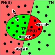
The left, and right, halves respectively contain instances that in fact have, and do not have, the condition. The oval contains instances that are classified (predicted) as positive (having the condition). Green and red respectively contain instances that are correctly (true), and wrongly (false), classified.
TP=True Positive; TN=True Negative; FP=False Positive (type I error); FN=False Negative (type II error); TPR=True Positive Rate; FPR=False Positive Rate; PPV=Positive Predictive Value; NPV=Negative Predictive Value.

When the classification function is not perfect, false results will appear. In the example confusion matrix below, of the 8 actual cats, a function predicted that three were dogs, and of the six dogs, it predicted that one was a rabbit and two were cats. We can see from the matrix that the system in question has trouble distinguishing between cats and dogs, but can make the distinction between rabbits and other types of animals pretty well.

Example confusion matrix
		Cat	Dog	Rabbit
		Predicted
Actual	Cat	5	3	0
	Dog	2	3	1
	Rabbit	0	2	11

False positives

False positives result when a test falsely (incorrectly) reports a positive result. For example, a medical test for a disease may return a positive result indicating that the patient has the disease even if the patient does not have the disease. False positive is commonly denoted as the top right (Condition negative X test outcome positive) unit in a Confusion matrix. We can use Bayes' theorem to determine the probability that a positive result is in fact a false positive. We find that if a disease is rare, then the majority of positive results may be false positives, even if the test is relatively accurate.

Suppose that a test for a disease generates the following results:

If a tested patient has the disease, the test returns a positive result 99% of the time, or with probability 0.99
If a tested patient does not have the disease, the test returns a positive result 5% of the time, or with probability 0.05.

Naively, one might think that only 5% of positive test results are false, but that is quite wrong, as we shall see.

Suppose that only 0.1% of the population has that disease, so that a randomly selected patient has a 0.001 prior probability of having the disease.

We can use Bayes' theorem to calculate the probability that a positive test result is a false positive.

Let A represent the condition in which the patient has the disease, and B represent the evidence of a positive test result. Then, the probability that the patient actually has the disease given the positive test result is

{\begin{aligned}P(A|B)&={\frac {P(B|A)P(A)}{P(B|A)P(A)+P(B|\neg A)P(\neg A)}}\\\\&={\frac {0.99\times 0.001}{0.99\times 0.001+0.05\times 0.999}}\\~\\&\approx 0.019.\end{aligned}}

and hence the probability that a positive result is a false positive is about 1 − 0.019 = 0.98, or 98%.

Despite the apparent high accuracy of the test, the incidence of the disease is so low that the vast majority of patients who test positive do not have the disease. Nonetheless, the fraction of patients who test positive who do have the disease (0.019) is 19 times the fraction of people who have not yet taken the test who have the disease (0.001). Thus the test is not useless, and re-testing may improve the reliability of the result.

In order to reduce the problem of false positives, a test should be very accurate in reporting a negative result when the patient does not have the disease. If the test reported a negative result in patients without the disease with probability 0.999, then

P(A|B)={\frac {0.99\times 0.001}{0.99\times 0.001+0.001\times 0.999}}\approx 0.5,

so that 1 − 0.5 = 0.5 now is the probability of a false positive.

False negatives

On the other hand, false negatives result when a test falsely or incorrectly reports a negative result. For example, a medical test for a disease may return a negative result indicating that patient does not have a disease even though the patient actually has the disease. False negative is commonly denoted as the bottom left (Condition positive X test outcome negative) unit in a Confusion matrix. We can also use Bayes' theorem to calculate the probability of a false negative. In the first example above,

{\begin{aligned}P(A|\neg B)&={\frac {P(\neg B|A)P(A)}{P(\neg B|A)P(A)+P(\neg B|\neg A)P(\neg A)}}\\\\&={\frac {0.01\times 0.001}{0.01\times 0.001+0.95\times 0.999}}\\~\\&\approx 0.0000105.\end{aligned}}

The probability that a negative result is a false negative is about 0.0000105 or 0.00105%. When a disease is rare, false negatives will not be a major problem with the test.

But if 60% of the population had the disease, then the probability of a false negative would be greater. With the above test, the probability of a false negative would be

{\begin{aligned}P(A|\neg B)&={\frac {P(\neg B|A)P(A)}{P(\neg B|A)P(A)+P(\neg B|\neg A)P(\neg A)}}\\\\&={\frac {0.01\times 0.6}{0.01\times 0.6+0.95\times 0.4}}\\~\\&\approx 0.0155.\end{aligned}}

The probability that a negative result is a false negative rises to 0.0155 or 1.55%.

True positives

True positives result when a tested truly (correctly) reports a positive result. As an example, a medical test for a disease may return a positive result indicating that the patient has the disease. This is shown to be true when the patient has the disease. True positive is commonly denoted as the top left (Condition positive X test outcome positive) unit in a Confusion matrix. We can use Bayes' theorem to determine the probability that the positive result is in fact a true positive using the example from above:

If a tested patient has the disease, the test returns a positive result 99% of the time, or with a probability of 0.99.
If a tested patient does not have the disease, the test returns a positive result 5% of the time, or with a probability of 0.05.
Suppose that only 0.1% of the population has that disease, so that a randomly selected patient has a 0.001 prior probability of having the disease.

Let A represent the condition in which the patient has the disease, and B represent the evidence of a positive test result. Then, the probability that the patient actually has the disease given a positive test result is:

{\begin{aligned}P(A|B)&={\frac {P(B|A)P(A)}{P(B|A)P(A)+P(B|\neg A)P(\neg A)}}\\\\&={\frac {0.99\times 0.001}{0.99\times 0.001+0.05\times 0.999}}\\~\\&\approx 0.019.\end{aligned}}

The probability that a positive result is a true positive is about 0.019%

True negatives

True negative result when a tested truly (correctly) reports a negative result. As an example, a medical test for a disease may return a positive result indicating that the patient does not have the disease. This is shown to be true when the patient does not have the disease. True negative is commonly denoted as the bottom right (Condition negative X test outcome negative) unit in a Confusion matrix.

We can also use Bayes' theorem to calculate the probability of true negative. Using the examples above:

If a tested patient has the disease, the test returns a positive result 99% of the time, or with a probability of 0.99.
If a tested patient does not have the disease, the test returns a positive result 5% of the time, or with a probability of 0.05.
Suppose that only 0.1% of the population has that disease, so that a randomly selected patient has a 0.001 prior probability of having the disease.

Let A represent the condition in which the patient has the disease, and B represent the evidence of a positive test result. Then, the probability that the patient actually has the disease given a positive test result is:

{\begin{aligned}P(A|\neg B)&={\frac {P(\neg B|A)P(A)}{P(\neg B|A)P(A)+P(\neg B|\neg A)P(\neg A)}}\\\\&={\frac {0.01\times 0.001}{0.01\times 0.001+0.95\times 0.999}}\\~\\&\approx 0.0000105.\end{aligned}}

The probability that a negative result is a true negative is 1 - 0.0000105 = 0.9999895 or 99.99%. Since the disease is rare and the positive to positive rate is high and the negative to negative rate is also high, this will produce a large True Negative rate.

Worked example

A worked example: A diagnostic test with sensitivity 67% and specificity 91% is applied to 2030 people to look for a disorder with a population prevalence of 1.48%

		Patients with bowel cancer (as confirmed on endoscopy)
		Condition positive	Condition negative	Prevalence = (TP + FN) / Total_Population = (20 + 10) / 2030 ≈ 1.48%	Accuracy (ACC) = (TP + TN) / Total_Population = (20 + 1820) / 2030 ≈ 90.64%
Fecal occult blood screen test outcome	Test outcome positive	True positive (TP) = 20 (2030 × 1.48% × 67%)	False positive (FP) = 180 (2030 × (100 − 1.48%) × (100 − 91%))	Positive predictive value (PPV), Precision = TP / (TP + FP) = 20 / (20 + 180) = 10%	False discovery rate (FDR) = FP / (TP + FP) = 180 / (20 + 180) = 90.0%
	Test outcome negative	False negative (FN) = 10 (2030 × 1.48% × (100 − 67%))	True negative (TN) = 1820 (2030 × (100 − 1.48%) × 91%)	False omission rate (FOR) = FN / (FN + TN) = 10 / (10 + 1820) ≈ 0.55%	Negative predictive value (NPV) = TN / (FN + TN) = 1820 / (10 + 1820) ≈ 99.45%
		TPR, Recall, Sensitivity = TP / (TP + FN) = 20 / (20 + 10) ≈ 66.7%	False positive rate (FPR),Fall-out, probability of false alarm = FP / (FP + TN) = 180 / (180 + 1820) = 9.0%	Positive likelihood ratio (LR+) = TPR/FPR = (20 / 30) / (180 / 2000) ≈ 7.41	Diagnostic odds ratio (DOR) = LR+/LR− ≈ 20.2	F₁ score = 2 × Precision × Recall/Precision + Recall ≈ 0.174
		False negative rate (FNR), Miss rate = FN / (TP + FN) = 10 / (20 + 10) ≈ 33.3%	Specificity, Selectivity, True negative rate (TNR) = TN / (FP + TN) = 1820 / (180 + 1820) = 91%	Negative likelihood ratio (LR−) = FNR/TNR = (10 / 30) / (1820 / 2000) ≈ 0.366

Related calculations

False positive rate (α) = type I error = 1 − specificity = FP / (FP + TN) = 180 / (180 + 1820) = 9%
False negative rate (β) = type II error = 1 − sensitivity = FN / (TP + FN) = 10 / (20 + 10) = 33%
Power = sensitivity = 1 − β
Positive likelihood ratio = sensitivity / (1 − specificity) = 0.67 / (1 − 0.91) = 7.4
Negative likelihood ratio = (1 − sensitivity) / specificity = (1 − 0.67) / 0.91 = 0.37
Prevalence threshold = $PT={\frac {{\sqrt {TPR(-TNR+1)}}+TNR-1}{(TPR+TNR-1)}}$ ≈ 0.2686 => 26.9%

This hypothetical screening test (fecal occult blood test) correctly identified two-thirds (66.7%) of patients with colorectal cancer.[lower-alpha 1] Unfortunately, factoring in prevalence rates reveals that this hypothetical test has a high false positive rate, and it does not reliably identify colorectal cancer in the overall population of asymptomatic people (PPV = 10%).

On the other hand, this hypothetical test demonstrates very accurate detection of cancer-free individuals (NPV = 99.5%). Therefore, when used for routine colorectal cancer screening with asymptomatic adults, a negative result supplies important data for the patient and doctor, such as ruling out cancer as the cause of gastrointestinal symptoms or reassuring patients worried about developing colorectal cancer.

Measuring a classifier with sensitivity and specificity

In training a classifier, one may wish to measure its performance using the well-accepted metrics of sensitivity and specificity. It may be instructive to compare the classifier to a random classifier that flips a coin based on the prevalence of a disease. Suppose that the probability a person has the disease is $p$ and the probability that they do not is $q=1-p$ . Suppose then that we have a random classifier that guesses that the patient has the disease with that same probability $p$ and guesses that he does not with the same probability $q$ .

The probability of a true positive is the probability that the patient has the disease times the probability that the random classifier guesses this correctly, or $p^{2}$ . With similar reasoning, the probability of a false negative is $pq$ . From the definitions above, the sensitivity of this classifier is $p^{2}/(p^{2}+pq)=p$ . With similar reasoning, we can calculate the specificity as $q^{2}/(q^{2}+pq)=q$ .

So, while the measure itself is independent of disease prevalence, the performance of this random classifier depends on disease prevalence. The classifier may have performance that is like this random classifier, but with a better-weighted coin (higher sensitivity and specificity). So, these measures may be influenced by disease prevalence. An alternative measure of performance is the Matthews correlation coefficient, for which any random classifier will get an average score of 0.

The extension of this concept to non-binary classifications yields the confusion matrix.

Notes

There are advantages and disadvantages for all medical screening tests. Clinical practice guidelines, such as those for colorectal cancer screening, describe these risks and benefits.[3][4]

References

Mathworld article for statistical test
Har-Peled, S., Roth, D., Zimak, D. (2003) "Constraint Classification for Multiclass Classification and Ranking." In: Becker, B., Thrun, S., Obermayer, K. (Eds) Advances in Neural Information Processing Systems 15: Proceedings of the 2002 Conference, MIT Press. ISBN 0-262-02550-7
Lin, Jennifer S.; Piper, Margaret A.; Perdue, Leslie A.; Rutter, Carolyn M.; Webber, Elizabeth M.; O’Connor, Elizabeth; Smith, Ning; Whitlock, Evelyn P. (21 June 2016). "Screening for Colorectal Cancer". JAMA. 315 (23): 2576–2594. doi:10.1001/jama.2016.3332. ISSN 0098-7484.
Bénard, Florence; Barkun, Alan N.; Martel, Myriam; Renteln, Daniel von (7 January 2018). "Systematic review of colorectal cancer screening guidelines for average-risk adults: Summarizing the current global recommendations". World Journal of Gastroenterology. 24 (1): 124–138. doi:10.3748/wjg.v24.i1.124. PMC 5757117. PMID 29358889.

This article is issued from Wikipedia. The text is licensed under Creative Commons - Attribution - Sharealike. Additional terms may apply for the media files.

[5] There are advantages and disadvantages for all medical screening tests. Clinical practice guidelines, such as those for colorectal cancer screening, describe these risks and benefits.[3][4]

[1] Mathworld article for statistical test

[2] Har-Peled, S., Roth, D., Zimak, D. (2003) "Constraint Classification for Multiclass Classification and Ranking." In: Becker, B., Thrun, S., Obermayer, K. (Eds) Advances in Neural Information Processing Systems 15: Proceedings of the 2002 Conference, MIT Press. ISBN 0-262-02550-7

[3] Lin, Jennifer S.; Piper, Margaret A.; Perdue, Leslie A.; Rutter, Carolyn M.; Webber, Elizabeth M.; O’Connor, Elizabeth; Smith, Ning; Whitlock, Evelyn P. (21 June 2016). "Screening for Colorectal Cancer". JAMA. 315 (23): 2576–2594. doi:10.1001/jama.2016.3332. ISSN 0098-7484.

[4] Bénard, Florence; Barkun, Alan N.; Martel, Myriam; Renteln, Daniel von (7 January 2018). "Systematic review of colorectal cancer screening guidelines for average-risk adults: Summarizing the current global recommendations". World Journal of Gastroenterology. 24 (1): 124–138. doi:10.3748/wjg.v24.i1.124. PMC 5757117. PMID 29358889.