Datar–Mathews method for real option valuation
The Datar–Mathews Method[1] (DM Method)[2] is a method for real options valuation. The method provides an easy way to determine the real option value of a project simply by using the average of positive outcomes for the project. The method can be understood as an extension of the net present value (NPV) multi-scenario Monte Carlo model with an adjustment for risk aversion and economic decision-making. The method uses information that arises naturally in a standard discounted cash flow (DCF), or NPV, project financial valuation. It was created in 2000 by Vinay Datar, professor at Seattle University; and Scott H. Mathews, Technical Fellow at The Boeing Company.
Method
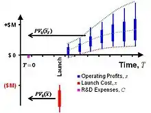
The mathematical equation for the DM Method is shown below. The method captures the real option value by discounting the distribution of operating profits at R, the market risk rate, and discounting the distribution of the discretionary investment at r, risk-free rate, before the expected payoff is calculated. The option value is then the expected value of the maximum of the difference between the two discounted distributions or zero.[3][4] Fig. 1.
- is a random variable representing the future benefits, or operating profits at time T. The present valuation of uses R, a discount rate consistent with the risk level of . R is the required rate of return for participation in the target market, sometimes termed the hurdle rate.
- is a random variable representing the strike price. The present valuation of uses r, the rate consistent with the risk of investment of . In many generalized option applications, the risk-free discount rate is used. However other discount rates can be considered, such as the corporate bond rate, particularly when the application is an internal corporate product development project.
- is the real option value for a single stage project. The option value can be understood as the expected value of the difference of two present value distributions with an economically rational threshold limiting losses on a risk-adjusted basis. This value may also be expressed as a stochastic distribution.
The differential discount rate for R and r implicitly allows the DM Method to account for the underlying risk.[5] If R > r, then the option will be risk-averse, typical for both financial and real options. If R < r, then the option will be risk-seeking. If R = r, then this is termed a risk-neutral option, and has parallels with NPV-type analyses with decision-making, such as decision trees. The DM Method gives the same results as the Black–Scholes and the binomial lattice option models, provided the same inputs and the discount methods are used. This non-traded real option value therefore is dependent on the risk perception of the evaluator toward a market asset relative to a privately held investment asset.
The DM Method is advantageous for use in real option applications because unlike some other option models it does not require a value for sigma (a measure of uncertainty) or for S0 (the value of the project today), both of which are difficult to derive for new product development projects; see further under real options valuation. Finally, the DM Method uses real-world values of any distribution type, avoiding the requirement for conversion to risk-neutral values and the restriction of a lognormal distribution;[6] see further under Monte Carlo methods for option pricing.
Extensions of the method for other real option valuations have been developed such as contract guarantee (put option), Multi-Stage (compound option), Early Launch (American option), and others.
Implementation
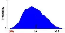
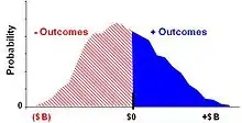
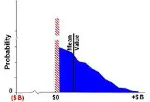
The DM Method may be implemented using Monte-Carlo simulation,[7] or in a simplified, algebraic or other form (see the DM Range Option below).
Using simulation, for each sample, the engine draws a random variable from both ST and XT, calculates their present values, and takes the difference.[8][9] Fig. 2A. The difference value is compared to zero, the maximum of the two is determined, and the resulting value recorded by the simulation engine. Here, reflecting the optionality inherent in the project, a forecast of a net negative value outcome corresponds to an abandoned project, and has a zero value.[10] Fig. 2B. The resulting values create a payoff distribution representing the economically rational set of plausible, discounted value forecasts of the project at time T0.
When sufficient payoff values have been recorded, typically a few hundred, then the mean, or expected value, of the payoff distribution is calculated. Fig. 2C. The option value is the expected value, the first moment of all positive NPVs and zeros, of the payoff distribution.[11]
A simple interpretation is:
where operating profit and launch costs are the appropriately discounted range of cash flows to time T0.[12]
Interpretation
Under certain constraints, the framework of a project investment problem structured for the Datar–Mathews Method can be converted to an equivalent framework structured for the Black–Scholes formula.[13] Fig. 3, Left. The Black–Scholes (as well as the binomial lattice) option pricing model is constrained to a lognormal distribution for the asset value, S, typical of traded financial options, and requires a scalar value for both S0 and XT, and sigma (σ0), a measure of volatility of the asset S. Assume a project investment problem with a forecasted lognormal asset value distribution with mean and standard deviation σT. The equivalent Black–Scholes values are:
The terms N(d1) and N(d2) are applied in the calculation of the Black–Scholes formula, and are expressions related to operations on lognormal distributions;[14] see section "Interpretation" under Black–Scholes. The Datar–Mathews Method does not use N(d1) or N(d2), but instead typically solves the option problem by means of Monte Carlo simulation applicable to many different types of distributions inherent in real option contexts. When the Datar–Mathews Method is applied to assets with lognormal distributions, it becomes possible to visualize graphically the operation of N(d1) and N(d2).

N(d2) is a measure of the area of the tail of the distribution relative to that of the entire distribution, e.g. the probability of tail of the distribution, at time T0. The tail of the distribution is delineated by X0 = XTe − rT, the present value of the strike price. Fig. 3, Right. The true probability of expiring in-the-money in the real (“physical”) world is calculated at time T, the launch date, measured by area of the tail of the distribution delineated by XT. N(d1) is the value of the option payoff relative to that of the asset; N(d1) = [MT × N(d2)]/S0, where MT is the mean of the tail at time T0. Using the DM Method, the value of a call option can be understood as C0 = (MT − X0) × N(d2).
DM Option
Algebraic form (Lognormal)
The DM Method can be extended to an algebraic form creating a generalized form for the DM Option. There are several advantages to the algebraic form, and ancillary simplifications, over the simulated approach as follows:
- Solves the option value explicitly
- Makes transparent the inner workings of option pricing technology
- Applies to many distribution types (lognormal, triangular, uniform, beta)[15]
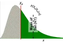
The algebraic form of the DM Option, whether modeled using a lognormal, triangular or other distribution, is fundamentally a simple concept and based on the same computation procedures. It is the conditional expectation of projected future value outcome distribution, , less a predetermined purchase cost (strike price or launch cost), , multiplied by the probability of that distribution. A conditional expectation is expected value of the truncated distribution (mean of the tail), MT, computed with respect to its conditional probability distribution[16] (Fig. 4).
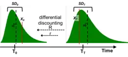
A financial option valuation (such as Black-Scholes) is based on a lognormal distribution projected from historical asset returns to present time T0 and using a lognormal distribution modeled by a volatility (finance) factor. A lognormal distribution is a close approximation to the distribution of traded financial asset returns. In contrast, real option valuation is based on a projection of a project’s future values at time TT, which may or may not be lognormally distributed. For comparison, the following real option example uses a lognormal distribution modeled using a standard deviation, SD, in place of the Black-Scholes volatility factor.
The valuation procedure values the project investment (option purchase, C0) at T0. The time differentiated discounting (R and r) results in an apparent shift of , or the mean , relative to the value outcome distribution, , or the mean (Fig. 5).[17][18] This relative shift sets up the conditional expectation of the truncated distribution at T0. Furthermore, the standard deviation, SD, of the distribution is proportionately discounted along with the distribution.
The standard deviation and mean of the non-logarithmized SD and S values are related to the logarithmic variance and mean, respectively, as:
The conditional expectation of the discounted value outcome is :
- is the cumulative distribution function of the standard normal distribution.
The probability of the project being in the money and launched (“exercised”) is
The project investment (option) value is:
Though similar in form to the Black-Scholes option value formula, the DM Option in algebraic form applies variables that are complementary with the structuring of a project valuation. By substituting the standard deviation for the volatility factor (specifically ), the two formulas can be shown to be equivalent.
Data patterns
The involved lognormal mathematics can be burdensome and opaque for some business practices within a corporation. However, several simplifications can ease that burden and provide clarity without sacrificing the soundness of the option calculation. One simplification is the employment of the standard normal distribution, also known as the Z-distribution, which has a mean of 0 and a standard deviation of 1. It is common practice to convert a normal distribution to a standard normal and then use the standard normal table to find the value of probabilities.
Define as the standard normal variable:
The conditional expectation of the discounted value outcome is:
Then probability of the project being in the money and launched (“exercised”) is:
The option value simplifies to:
Businesses that collect historical data may be able to leverage the similarity of assumptions across related projects facilitating the calculation of option values. One resulting simplification is the Uncertainty Ratio, , which can often be modeled as a constant for similar projects. UR is the degree of certainty by which the projected future cash flows can be estimated. UR is invariant of time with values typically between 0.35 and 1.0 for many multi-year business projects.
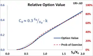
Applying this observation as a constant, K, to the above formulas results in a simpler formulation:
The resulting real option value can be derived simply on a hand-held calculator once K is determined:
| Variables | S0N(K-Z)-X0N(-Z) | S0(0.31S0/X0-0.10) |
|---|---|---|
| UR / K | 0.6 / 0.55 | |
| S0/X0 | 1.0 | 1.0 |
| Z | 0.28 | |
| S0 | $10.0M | $10.0M |
| C0 | $2.18M | $2.10M |
| Difference | 4% | |
Assuming the UR is held constant, then the relative value of the option is determined by the ratio of , which is proportional to the probability of the project being in the money and launched (exercised). Then (Fig. 6) Businesses need apply their own data across similar projects to establish relevant parameter values.
As an additional check on estimating operating profits () with uncertainty, an example of results in a value range of:
A value range of approximately an order of magnitude may seem large, even excessive. However, a real option business case is most often applied to multi-year early-stage projects that embody large uncertainties, which therefore is reflected with a wide estimated value range representing worst-to-best case scenarios.
DM Range Option – (Triangular)
Given the difficulty in estimating the lognormal distribution mean and standard deviation of future returns, other distributions instead are more often applied for real options used in business decision making. The sampled distributions may take any form, although the triangular distribution is often used, as is typical for low data situations, followed by a uniform distribution (continuous) or a beta distribution.[19][20] This approach is useful for early-stage estimates of project option value when there has not been sufficient time or resources to gather the necessary quantitative information required for a complete cash flow simulation, or in a portfolio of projects when simulation of all the projects is too computationally demanding.[21] Regardless of the distribution chosen, the procedure remains the same for a real option valuation.
| Innovation Project Quick Contingent Value Estimate |
With most likely PV operating cash flow of $8.5M, but a 3-year capital cost of roughly $20M, the NPV of the important innovation project was deeply negative and the manager is considering abandoning it. Corporate sales analytics estimated with 95% certainty (double-sided 1-in-10 chance) the revenues could be as low as $4M or as high as $34M. (Fig. 8) Because of the large potential upside, the manager believes a small initial investment might resolve the project's downside uncertainties and reveal its potential value.[22] 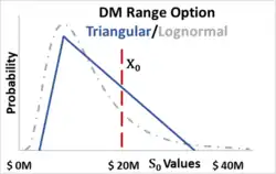 Fig. 8 DM Range Option with triangular distribution. (Background: comparable lognormal distribution.) Using the DM Range Option as a guide, the manager calculated the expected contingent value of the project upside to be about $25M [≈ (2*$20M + $34M)/3]. Furthermore, there is a probability of one-in-four {25% ≈ ($34M - $20M)2 /[ ($34M - $4M)($34M-$8.5M)]} that the project revenues will be greater than $20M. With these calculations, the manager estimates the innovation project option value is $1.25M [= ($25M-$20M) * 25%]. Using this value, the manager justifies this initial investment (about 6% of the capital cost) into the project, sufficient to resolve some of the key uncertainties. The project can always be abandoned should the intermediate development results not measure up, but the investment losses will be minimized. (Later using corporate historical data patterns, an analyst converted the values from a three-point estimate to a DM Option calculation, and demonstrated that the result would differ by less than 10%.) |
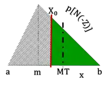
For a triangular distribution, sometimes referred to as three-point estimation, the mode value corresponds to the “most-likely” scenario, and the other two other scenarios, “pessimistic” and “optimistic”, represent plausible deviations from the most-likely scenario (often modeled as approximating a two-sided 1-out-of-10 likelihood or 95% confidence).[23][24][25][26] This range of estimates results in the eponymous name for the option, the DM Range Option.[27] The DM Range Option method is similar to the fuzzy method for real options. The following example (Fig. 7) uses a range of future estimated operating profits of a (pessimistic), b (optimistic) and m (mode or most-likely).
For discount a, b and m by
The classic DM Method presumes that the strike price is represented by a random variable (distribution ) with the option solution derived by simulation. Alternatively, without the burden of performing a simulation, applying the average or mean scalar value of the launch cost distribution (strike price) results in a conservative estimate of DM Range Option value. If the launch cost is predetermined as a scalar value, then the DM Range Option value calculation is exact.
The expected value of the truncated triangular distribution (mean of the right tail), is
The probability of the project being in the money and launched is the proportional area of the truncated distribution relative to the complete triangular distribution. This partial expectation is computed by the cumulative distribution function (CDF) given the probability distribution will be found at a value greater than or equal to X:
The DM Range Option value, or project investment, is:
The values of the triangular distribution can be estimated to those of the logarithmic distribution by using a range within standard deviations of its mean (≈95% confidence) as follows:
Use of a DM Range Option facilitates the application of real option valuation to future project investments. The DM Range Option provides an estimate of valuation that differs marginally with that of the DM Option algebraic lognormal distribution form. However, the projected future value outcome, S, of a project is rarely based on a lognormal distribution derived from historical asset returns, as is a financial option. Rather, the future value outcome, S, (as well as the strike price, X, and the standard deviation, SD), is more than likely a three-point estimation based on engineering and marketing parameters. Therefore, the ease of application of the DM Range Option is often justified by its expediency and is sufficient to estimate the conditional value of a future project.
Comparison to other methods
In a 2016 article in the Advances in Decision Sciences journal, researchers from the Lappeenranta University of Technology School of Business and Management compared the DM Method to the fuzzy pay-off method for real option valuation created in 2009, and noted that while the valuation results were similar, the fuzzy pay-off one was more robust in some conditions.[28] In some comparative cases, Datar-Mathews Method has a significant advantage in that it is easier to operate and connects NPV valuation and scenario analysis with Monte Carlo simulation technique thus greatly improving intuition in the usage of real options methods in managerial decision and explain to third parties.[29] Through its simulation interface, the Datar-Mathews Method easily accommodates multiple and sometimes correlated cash flow scenarios, including dynamic programming, typical of complex projects, such as aerospace, that are difficult to model using fuzzy sets.[30]
References
- Mathews, Scott; Datar, Vinay; Johnson, Blake (2007). "A Practical Method for Valuing Real Options: The Boeing Approach". Journal of Applied Corporate Finance. 19 (2): 95–104. doi:10.1111/j.1745-6622.2007.00140.x.
- U.S. Patent No. 6,862,579 (issued March 1, 2005).
- Nugroho, Lukito Adi; McMillan, David (28 April 2017). "Real options valuation of franchise territorial exclusivity". Cogent Business & Management. 4 (1): 4–5. doi:10.1080/23311975.2016.1262490.
- Barton, Kelsey; Lawryshyn, Yuri (2010-06-17). Reconciling Real Option Models: An Approach to Incorporate Market and Private Uncertainties (PDF). Real Options: Theory Meets Practice - 14th Annual International Conference. Rome, Italy.
- Savolainen, Jyrki; Collan, Mikael; Luukka, Pasi (2016). "Combining System Dynamic Modeling and the Datar–Mathews Method for Analyzing Metal Mine Investments". Acta Universitatis Palackianae Olomucensis. Facultas Rerum Naturalium. Mathematica. 55 (1): 95–110. hdl:10338.dmlcz/145821. ISSN 0231-9721.
- Datar, Vinay T. and Mathews, Scott H., 2004. European Real Options: An Intuitive Algorithm for the Black–Scholes Formula. Journal of Applied Finance 14(1): 7–13
- Brigatti, E; Macias F.; Souza M.O.; Zubelli J.P. (2015). Aid, R (ed.). A Hedged Monte Carlo Approach to Real Option Pricing. New York, NY: Springer. p. 7. arXiv:1509.03577. doi:10.1007/978-1-4939-2733-3_10. ISBN 978-1-4939-2733-3.
- Business Engineering: A Practical Approach to Valuing High-Risk, High-Return Projects Using Real Options Tutorials in Operations Research 2007, Operations Research Tools and Applications: Glimpses of Future Technologies, p157–175
- Business Engineering: A Practical Approach to Valuing High-Risk, High-Return Projects Using Real Options INFORMS Annual Meeting, November 4–7, 2007
- Baldwin, Dr. Samuel F., Chief Scientist for the Office of Energy Efficiency and Renewable Energy (2015-03-04). Chapter 12: Integrated Analysis 2.4 Flexible Decision Making (11) (Speech). Quadrennial Technology Review. U.S. Department of Energy (DOE).
- Kozlova, Mariia (April 2015). Analyzing the Effects of the New Renewable Energy Policy in Russia on Investments into Wind, Solar and Small Hydro Power (Thesis). Lappeenranta University of Technology. pp. 62–66.
- Mathews, Scott H., 2009. Tutorial CIFER-T2 Boeing's method for valuing high-risk high-return technology projects using real options. IEEE Symposium on Computational Intelligence for Financial Engineering, 2009.
- Collan, Mikael (2011). "Thoughts about Selected Models for the Valuation of Real Options". Acta Universitatis Palackianae Olomucensis. Facultas Rerum Naturalium. Mathematica. 50 (2): 5–12. ISSN 0231-9721.
- Don Chance (2011). Derivation and Interpretation of the Black–Scholes Model.
- Vedernikov, Andrei (2016). Valuing Synergies in Strategic Acquisitions using Real Options (PDF) (Thesis). St. Petersburg University, Graduate School of Management.
- Gyoshev, Stanley B.; Gombola, Michael (2012-12-04). "A Separating Equilibrium for Stock Repurchase Programs via PUT Options: Transforming a Mathematical Proof into Visual Form". SSRN Working Paper Series: 4, 17. doi:10.2139/ssrn.2185093. ISSN 1556-5068.
- Luenberger, David (Autumn 1998). "The Two-Rate Method of Discounting". Investment Science Newsletter. Department of Management Science & Engineering, Stanford University. Retrieved 2019-11-08.
- Justin, Cedric Yves; Mavris, Dimitri N. (2011-09-20). Option-Based Approach to Value Engine Maintenance Cost Guarantees and Engine Maintenance Contracts. 11th AIAA Aviation Technology, Integration, and Operations (ATIO) Conference. p. 7. doi:10.2514/6.2011-6839.
- Alabi, Olabode (2010-04-30). Evaluation Method for Strategic Investments (Dissertation). University of Nebraska - Lincoln.
- Peters, Linda (September 2016). "Impact of Probability Distributions on Real Options Valuation". Journal of Infrastructure Systems. 22 (3): 04016005. doi:10.1061/(ASCE)IS.1943-555X.0000289. hdl:10067/1319100151162165141. S2CID 56465582.
- Innovation Portfolio Architecture – Part 2: Attribute Selection and Valuation Archived 2014-08-30 at the Wayback Machine. Research-Technology Management Vol. 54, No. 5 September–October 2011
- Sadowsky, Jeffery R. (May 10, 2005). "The Value of Learning in the Product Development Stage: A Real Options Approach". SSRN: 9. doi:10.2139/ssrn.721597. S2CID 12742583.
- Mathews, Scott (2010). "Valuing High-Risk High-Return technology Projects Using Real Options". In Bidgoli, Hossein (ed.). The Handbook of Technology Management: Core Concepts, Financial Tools and Techniques, Operations and Innovation Management. 1. Hoboken, NJ: Wiley. pp. 581–600. ISBN 978-0470249475.
- Onkham, Wilawan (2013). A Real Option Dynamic Decision Framework for Operational Innovations (PhD). University of Central Florida. p. 44.
- Naedele, Martin; Chen, Hong-Mei; Kazman, Rick; Cai, Yuanfang; Xiao, Lu; Silva, Carlos V.A. (March 2015). "Manufacturing execution systems: A vision for managing software development". Journal of Systems and Software. 101: 59–68. doi:10.1016/j.jss.2014.11.015.
- Patregnani, Giulia (2014-10-13). The Value of Synergies through the Real Options Lenses (Graduate Theses, MS in Finance and Strategic Management). Copenhagen School of Business. pp. 63–65. hdl:10417/4840.
- Mathews, Scott (September–October 2009). "Valuing Risky Projects with Real Options". Research Technology Management. 52 (5): 32–41. doi:10.1080/08956308.2009.11657587. JSTOR 43240438.
- https://www.hindawi.com/journals/ads/2016/7836784/
- Loukianova, Anna; Nikulin, Egor; Vedernikov, Andrey (12 May 2017). "Valuing synergies in strategic mergers and acquisitions using the real options approach". Investment Management and Financial Innovations. 14 (1): 236–247. doi:10.21511/imfi.14(1-1).2017.10.
- Schachter, Jonathan A. Schachter (2016). A Real Options Approach to Valuing Flexibility in Demand-Side Response Operations and Investments under Uncertainty (PhD). The University of Manchester. Retrieved 2016-08-01.
