Earned schedule
Earned schedule (ES) is an extension to the theory and practice of earned value management (EVM).
It has been stated that Earned Schedule provides a useful link between traditional Earned Value Analysis and traditional project schedule analysis -- a link that some say has been missing in traditional EVM theory.
Earned schedule measures
Traditionally, EVM tracks schedule variances not in units of time, but in units of currency (e.g. dollars) or quantity (e.g. labor hours). Of course, it is more natural to speak of schedule performance in units of time, but the problems with traditional schedule performance metrics are even deeper. Near the end of a project -- when schedule performance is often a primary concern -- the usefulness of traditional schedule metrics is demonstrably poor. When a project is completed, its SV is always 0 and SPI is always 1, even if the project was delivered unacceptably late. Similarly, a project can languish near completion (e.g. SPI = 0.95) and never be flagged as outside acceptable numerical tolerance. (Using traditional SV as an exception threshold, it is not uncommon that an SPI > 0.9 is considered acceptable.)
To correct these problems, Earned Schedule theory represents the two measures SV and SPI in 2 separate domains: currency and time. They are named as SV($) and SPI($), to indicate they relate to currency; and SV(t) and SPI(t), to indicate they relate to time.
A stated advantage of Earned Schedule methods is that no new data collection processes are required to implement and test Earned Schedule; it only requires updated formulas. Earned Schedule theory also provides updated formulas for predicting project completion date, using the time-based measures.
As emerging practice
As of 2005, Earned Schedule is designated as an "emerging practice" by the Project Management Institute. It was introduced in 2003 a seminal article "Schedule is Different" [1] by Walter Lipke, in The Measurable News, the quarterly magazine of the College of Performance Management, of the Project Management Institute.
Limitation
In spite of more than a decade using Earned Schedule, the general appreciation to that was less than it was expected. One of the most significant reasons of this occurrence is the great difference of forecasting one period from the other periods. For instance note the following table. The following information was gained from the documents of final processes of a completed project which depicts the results of applying the new index in various time periods.
| 1226 | 1136 | 1046 | 956 | 866 | 776 | 686 | 596 | AT |
| 1283 | 1283 | 1283 | 1283 | 1283 | 1283 | 1283 | 1283 | AD |
| 1236 | 1564 | 2884 | 2233 | 2799 | 3574 | 3465 | 3665 | IEAC(t) |
AT in which is a day the report is prepared and AD is the actual time been spent on the completion of operating the project. As it is noticed, the more we get close to the actual completion of the project (AD=1283), the presented results get more realistic. However the variance in different time estimate in is notable. For instance the estimate at the end of the sixth period has the discrepancy of more than 1000 days with the estimate at the end of the seventh day however there is a gap of only 90 days between these two periods. The most important feedback of such a problem may vary from the distrust of stakeholders of management reports to their changing their turnabout to proceed with the project (considering the estimate of the sixth period). Concerning this issue, while investigating the way to calculate the mentioned index, we decided to evaluate its conformity to the gained actuality. In order to do so, the planned and actual graph of progress of the project has been considered.
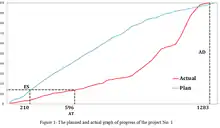
ES = 210
AD = 1283
AT = 596
IEAC(t) = 3665
Since the amount of AD in all the reported forecasts is similar, it can be concluded that the estimates are relevant to the reverse of schedule performance index of time (SPI ((T)). In better words, independent estimation at completion (IEAC (T)) is calculated based on schedule performance index at the moment of “t”. Unaware of the fact that the actual progress at the moment “t” can have an illogical ascending performance, affected by the sharp decline of budget, the unusual descending performance or increase of human resource at a certain time.
In addition, given that in order to calculate ES, the actual progress curve is depicted on planned progress curve. Forecasting the future condition of the project is based on the assumption that all the next periods will encounter the deviation from the schedule based on the current amount SPI (T). While with the assumption of making special conditions, the mentioned index may be reported more or less because of the illogical reasons. For instance if at the point AT= 626 we forecasted the future of the project, the following information would be gained:
ES = 243
AD = 1283
AT = 626
IEAC(t) = 3376
However the study on the condition of progress around this point shows that this condition had a sudden growth at the end of 2013 only due to the injection of budget. Thus, the first problem of the method ES can be known as the ignoring the actual progress of curve performance in predicting the future condition.
Because of that problem, the new method which is named "Forecasting at completion" had presented in Industrial Engineering and Operation Management conference (IEOM 2019). This method is base on linear regression and polynomial regression. [2]
Notes and references
- Lipke, Walt (2003). "Schedule Is Different" (PDF). Project Management Institute College of Performance Management.
- Maaleki, Ali. "Forecasting at Completion: Introduction of New Method and Comparing It with the Method of Earned Schedule" (PDF).
