Falkner–Skan boundary layer

A schematic diagram of the Blasius flow profile. The streamwise velocity component ${\displaystyle u(\eta )/U(x)}$ is shown, as a function of the similarity variable ${\displaystyle \eta }$.

Prandtl's[2] equations known as the boundary layer equations for steady incompressible flow with constant viscosity and density, are

${\displaystyle {\dfrac {\partial u}{\partial x}}+{\dfrac {\partial v}{\partial y}}=0}$

${\displaystyle u{\dfrac {\partial u}{\partial x}}+v{\dfrac {\partial u}{\partial y}}=-{\dfrac {1}{\rho }}{\dfrac {\partial p}{\partial x}}+{\nu }{\dfrac {\partial ^{2}u}{\partial y^{2}}}}$

${\displaystyle {\dfrac {\partial p}{\partial y}}=0}$

Here the coordinate system is chosen with ${\displaystyle x}$ pointing parallel to the plate in the direction of the flow and the ${\displaystyle y}$ coordinate pointing towards the free stream, ${\displaystyle u}$ and ${\displaystyle v}$ are the ${\displaystyle x}$ and ${\displaystyle y}$ velocity components, ${\displaystyle p}$ is the pressure, ${\displaystyle \rho }$ is the density and ${\displaystyle \nu }$ is the kinematic viscosity.

The ${\displaystyle y}$-momentum equation implies that the pressure in the boundary layer must be equal to that of the free stream for any given ${\displaystyle x}$ coordinate. Because the velocity profile is uniform in the free stream, there is no vorticity involved, therefore a simple Bernoulli's equation can be applied in this high Reynolds number limit ${\displaystyle {\dfrac {p}{\rho }}+{\dfrac {U^{2}}{2}}=}$ constant or, after differentiation: ${\displaystyle {\dfrac {1}{\rho }}{\dfrac {dp}{dx}}=-U{\dfrac {dU}{dx}}}$ Here ${\displaystyle U(x)}$ is the velocity of the fluid outside the boundary layer and is a solution of Euler equations (fluid dynamics).

A number of similarity solutions to this equation have been found for various types of flow, including flat plate boundary layers. The term similarity refers to the property that the velocity profiles at different positions in the flow are the same apart from a scaling factor. These solutions are often presented in the form of non-linear ordinary differential equations.

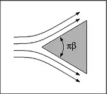
We can generalize the Blasius boundary layer by considering a wedge at an angle of attack ${\displaystyle \pi \beta /2}$ from some uniform velocity field ${\displaystyle U_{0}}$. We then estimate the outer flow to be of the form:

${\displaystyle u_{e}(x)=U_{0}\left({\frac {x}{L}}\right)^{m}}$

Where ${\displaystyle L}$ is a characteristic length and m is a dimensionless constant. In the Blasius solution, m = 0 corresponding to an angle of attack of zero radians. Thus we can write:

${\displaystyle \beta ={\frac {2m}{m+1}}.}$

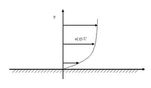
As in the Blasius solution, we use a similarity variable ${\displaystyle \eta }$ to solve the boundary layer equations.

Falkner-Skan boundary layer profiles for selected values of ${\displaystyle m}$.

${\displaystyle \eta =y{\sqrt {\frac {U_{0}(m+1)}{2\nu L}}}\left({\frac {x}{L}}\right)^{(m-1)/2}}$

It becomes easier to describe this in terms of its stream function which we write as

${\displaystyle \psi =U(x)\delta (x)f(\eta )={\sqrt {\frac {2\nu U_{0}L}{m+1}}}\left({\frac {x}{L}}\right)^{(m+1)/2}f(\eta )}$

Thus the initial differential equation which was written as follows:

${\displaystyle u{\partial u \over \partial x}+v{\partial u \over \partial y}=c^{2}mx^{2m-1}+{\nu }{\partial ^{2}u \over \partial y^{2}}.}$

Can now be expressed in terms of the non-linear ODE known as the Falkner–Skan equation.

${\displaystyle f'''+ff''+\beta \left[1-(f')^{2}\right]=0}$

with boundary conditions

${\displaystyle f(0)=f'(0)=0,\quad f'(\infty )=1.}$

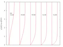
When ${\displaystyle \beta =1}$, the problem reduces to the Hiemenz flow. Here, m < 0 corresponds to an adverse pressure gradient (often resulting in boundary layer separation) while m > 0 represents a favorable pressure gradient. (Note that m = 0 recovers the Blasius equation). In 1937 Douglas Hartree showed that physical solutions to the Falkner–Skan equation exist only in the range ${\displaystyle -0.090429\leq m\leq 2\ (-0.198838\leq \beta \leq 4/3)}$. For more negative values of m, that is, for stronger adverse pressure gradients, all solutions satisfying the boundary conditions at η = 0 have the property that f(η) > 1 for a range of values of η. This is physically unacceptable because it implies that the velocity in the boundary layer is greater than in the main flow.[4]

Further details may be found in Wilcox (2007).

The displacement thickness for the Falkner-Skan profile is given by

${\displaystyle \delta =\left({\frac {2}{m+1}}\right)^{1/2}\left({\frac {\nu x}{U}}\right)^{1/2}\int _{0}^{\infty }(1-f')d\eta }$

and the shear stress acting at the wedge is given by

${\displaystyle \tau _{w}=\mu \left({\frac {m+1}{2}}\right)^{1/2}\left({\frac {U^{3}}{\nu x}}\right)^{1/2}f''(0)}$

Here Falkner–Skan boundary layer with a specified specific enthalpy ${\displaystyle h}$ at the wall is studied. The density ${\displaystyle \rho }$, viscosity ${\displaystyle \mu }$ and thermal conductivity ${\displaystyle \kappa }$ are no longer constant here. In the low Mach number approximation, the equation for conservation of mass, momentum and energy become

${\displaystyle {\begin{aligned}{\frac {\partial (\rho u)}{\partial x}}+{\frac {\partial (\rho v)}{\partial y}}&=0,\\\rho \left(u{\frac {\partial u}{\partial x}}+v{\frac {\partial u}{\partial y}}\right)&=-{\frac {1}{\rho }}{\frac {dp}{dx}}+{\frac {\partial }{\partial y}}\left(\mu {\frac {\partial u}{\partial y}}\right),\\\rho \left(u{\frac {\partial h}{\partial x}}+v{\frac {\partial h}{\partial y}}\right)&={\frac {\partial }{\partial y}}\left({\frac {\mu }{Pr}}{\frac {\partial h}{\partial y}}\right)\end{aligned}}}$

where ${\displaystyle Pr=c_{p_{\infty }}\mu _{\infty }/\kappa _{\infty }}$ is the Prandtl number with suffix ${\displaystyle \infty }$ representing properties evaluated at infinity. The boundary conditions become

${\displaystyle u=v=h-h_{w}(x)=0\ {\text{for}}\ y=0}$,

${\displaystyle u-U=h-h_{\infty }=0\ {\text{for}}\ y=\infty \ {\text{or}}\ x=0}$.

Unlike the incompressible boundary layer, similarity solution can exists for only if the transformation

${\displaystyle x\rightarrow c^{2}x,\quad y\rightarrow cy,\quad u\rightarrow u,\quad v\rightarrow {\frac {v}{c}},\quad h\rightarrow h,\quad \rho \rightarrow \rho ,\quad \mu \rightarrow \mu }$

holds and this is possible only if ${\displaystyle h_{w}={\text{constant}}}$.

• Blasius boundary layer

References

- V. M. Falkner and S. W. Skan, Aero. Res. Coun. Rep. and Mem. no 1314, 1930.
- Prandtl, L. (1904). "Über Flüssigkeitsbewegung bei sehr kleiner Reibung". Verhandlinger 3. Int. Math. Kongr. Heidelberg: 484–491.
- Rosenhead, Louis, ed. Laminar boundary layers. Clarendon Press, 1963.
- Stewartson, K. (3 December 1953). "Further Solutions of the Falkner-Skan Equation" (PDF). Mathematical Transactions of the Cambridge Philosophical Society. 50 (3): 454–465. doi:10.1017/S030500410002956X. Retrieved 2 March 2017.
- Lagerstrom, Paco Axel. Laminar flow theory. Princeton University Press, 1996.