Hopfield network

Ising model of a neural network as a memory model is first proposed by William A. Little in 1974.[5]

A Hopfield net with four units

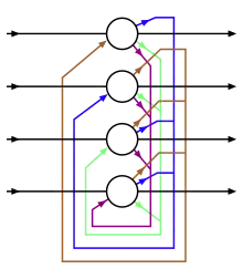
The units in Hopfield nets are binary threshold units, i.e. the units only take on two different values for their states and the value is determined by whether or not the units' input exceeds their threshold ${\displaystyle U_{i}}$. Discrete Hopfield nets describe relationships between binary (firing or not-firing) neurons ${\displaystyle 1,2,...i,j,...N}$.[6] At a certain time, the state of the neural net is described by a vector ${\displaystyle V}$, which records which neurons are firing in a binary word of N bits.

The interactions ${\displaystyle w_{ij}}$ between neurons have units that usually take on values of 1 or -1, and this convention will be used throughout this article. However, other literature might use units that take values of 0 and 1. These interactions are "learned" via Hebb's law of association, such that, for a certain state ${\displaystyle V^{s}}$

${\displaystyle w_{ij}=(2V_{i}^{s}-1)(2V_{j}^{s}-1)}$

but ${\displaystyle w_{ii}=0}$. The neural net acts on neurons such that

• ${\displaystyle V_{i}\rightarrow 1}$ if ${\displaystyle \sum _{j}w_{ij}V_{j}>U_{i}}$
• ${\displaystyle V_{i}\rightarrow 0}$ if ${\displaystyle \sum _{j}w_{ij}V_{j}<U_{i}}$

In this way, Hopfield networks have the ability to "remember" states stored in the interaction matrix, because if a new state ${\displaystyle V^{s'}}$ is subjected to the interaction matrix, each neuron will change until it matches the original state ${\displaystyle V^{s}}$ (see the Updates section below).

The connections in a Hopfield net typically have the following restrictions:

• ${\displaystyle w_{ii}=0,\forall i}$ (no unit has a connection with itself)
• ${\displaystyle w_{ij}=w_{ji},\forall i,j}$ (connections are symmetric)

The constraint that weights are symmetric guarantees that the energy function decreases monotonically while following the activation rules.[7] A network with asymmetric weights may exhibit some periodic or chaotic behaviour; however, Hopfield found that this behavior is confined to relatively small parts of the phase space and does not impair the network's ability to act as a content-addressable associative memory system.

Hopfield also modeled neural nets for continuous values, in which the electric output of each neuron is not binary but some value between 0 and 1.[8] He found that this type of network was also able to store and reproduce memorized states.

Notice that every pair of units i and j in a Hopfield network has a connection that is described by the connectivity weight ${\displaystyle w_{ij}}$. In this sense, the Hopfield network can be formally described as a complete undirected graph ${\displaystyle G=\langle V,f\rangle }$, where ${\displaystyle V}$ is a set of McCulloch–Pitts neurons and ${\displaystyle f:V^{2}\rightarrow \mathbb {R} }$ is a function that links pairs of units to a real value, the connectivity weight.

Updating one unit (node in the graph simulating the artificial neuron) in the Hopfield network is performed using the following rule:

${\displaystyle s_{i}\leftarrow \left\{{\begin{array}{ll}+1&{\mbox{if }}\sum _{j}{w_{ij}s_{j}}\geq \theta _{i},\\-1&{\mbox{otherwise.}}\end{array}}\right.}$

where:

• ${\displaystyle w_{ij}}$ is the strength of the connection weight from unit j to unit i (the weight of the connection).
• ${\displaystyle s_{i}}$ is the state of unit i.
• ${\displaystyle \theta _{i}}$ is the threshold of unit i.

Updates in the Hopfield network can be performed in two different ways:

• Asynchronous: Only one unit is updated at a time. This unit can be picked at random, or a pre-defined order can be imposed from the very beginning.
• Synchronous: All units are updated at the same time. This requires a central clock to the system in order to maintain synchronization. This method is viewed by some as less realistic, based on an absence of observed global clock influencing analogous biological or physical systems of interest.

Bruck shed light on the behavior of a neuron in the discrete Hopfield network when proving its convergence in his paper in 1990.[9]  A subsequent paper [10] further investigated the behavior of any neuron in both discrete-time and continuous-time Hopfield networks when the corresponding energy function is minimized during an optimization process. Bruck shows[9] that neuron j changes its state if and only if it further decreases the following biased pseudo-cut. The discrete Hopfield network minimizes the following biased pseudo-cut [10] for the synaptic weight matrix of the Hopfield net.

${\displaystyle J_{pseudo-cut}(k)=\sum _{i\in C_{1}(k)}\sum _{j\in C_{2}(k)}w_{ij}+\sum _{j\in C_{1}(k)}{\theta _{j}}}$

where ${\displaystyle C_{1}(k)}$ and ${\displaystyle C_{2}(k)}$ represents the set of neurons which are -1 and +1, respectively, at time ${\displaystyle k}$. For further details, see the recent paper.[10]

The discrete-time Hopfield Network always minimizes exactly the following pseudo-cut   (,[9][10])

${\displaystyle U(k)=\sum _{i=1}^{N}\sum _{j=1}^{N}w_{ij}(s_{i}(k)-s_{j}(k))^{2}+2\sum _{j=1}^{N}{\theta _{j}}s_{j}(k)}$

The continuous-time Hopfield network always minimizes an upper bound to the following weighted cut  [10]

${\displaystyle V(t)=\sum _{i=1}^{N}\sum _{j=1}^{N}w_{ij}({f(s_{i}(t))}-f(s_{j}(t))^{2}+2\sum _{j=1}^{N}{\theta _{j}}{f(s_{j}(t))}}$

where ${\displaystyle f(.)}$ is a zero-centered sigmoid function.

The complex Hopfield network, on the other hand, generally tends to minimize the so-called shadow-cut of the complex weight matrix of the net.[11]

Energy Landscape of a Hopfield Network, highlighting the current state of the network (up the hill), an attractor state to which it will eventually converge, a minimum energy level and a basin of attraction shaded in green. Note how the update of the Hopfield Network is always going down in Energy.

Hopfield nets have a scalar value associated with each state of the network, referred to as the "energy", E, of the network, where:

${\displaystyle E=-{\frac {1}{2}}\sum _{i,j}{w_{ij}{s_{i}}{s_{j}}}+\sum _{i}{\theta _{i}}{s_{i}}}$

This quantity is called "energy" because it either decreases or stays the same upon network units being updated. Furthermore, under repeated updating the network will eventually converge to a state which is a local minimum in the energy function (which is considered to be a Lyapunov function).[6] Thus, if a state is a local minimum in the energy function it is a stable state for the network. Note that this energy function belongs to a general class of models in physics under the name of Ising models; these in turn are a special case of Markov networks, since the associated probability measure, the Gibbs measure, has the Markov property.

Hopfield and Tank presented the Hopfield network application in solving the classical traveling-salesman problem in 1985.[12] Since then, the Hopfield network has been widely used for optimization. The idea of using the Hopfield network in optimization problems is straightforward: If a constrained/unconstrained cost function can be written in the form of the Hopfield energy function E, then there exists a Hopfield network whose equilibrium points represent solutions to the constrained/unconstrained optimization problem.  Minimizing the Hopfield energy function both minimizes the objective function and satisfies the constraints also as the constraints are “embedded” into the synaptic weights of the network. Although including the optimization constraints into the synaptic weights in the best possible way is a challenging task, indeed many various difficult optimization problems with constraints in different disciplines have been converted to the Hopfield energy function: Associative memory systems, Analog-to-Digital conversion, job-shop scheduling problem, quadratic assignment and other related NP-complete problems, channel allocation problem in wireless networks, mobile ad-hoc network routing problem, image restoration, system identification, combinatorial optimization, etc, just to name a few. Further details can be found in e.g. the paper.[10]  

Initialization of the Hopfield networks is done by setting the values of the units to the desired start pattern. Repeated updates are then performed until the network converges to an attractor pattern. Convergence is generally assured, as Hopfield proved that the attractors of this nonlinear dynamical system are stable, not periodic or chaotic as in some other systems. Therefore, in the context of Hopfield networks, an attractor pattern is a final stable state, a pattern that cannot change any value within it under updating.

Training a Hopfield net involves lowering the energy of states that the net should "remember". This allows the net to serve as a content addressable memory system, that is to say, the network will converge to a "remembered" state if it is given only part of the state. The net can be used to recover from a distorted input to the trained state that is most similar to that input. This is called associative memory because it recovers memories on the basis of similarity. For example, if we train a Hopfield net with five units so that the state (1, -1, 1, -1, 1) is an energy minimum, and we give the network the state (1, -1, -1, -1, 1) it will converge to (1, -1, 1, -1, 1). Thus, the network is properly trained when the energy of states which the network should remember are local minima. Note that, in contrast to Perceptron training, the thresholds of the neurons are never updated.

Patterns that the network uses for training (called retrieval states) become attractors of the system. Repeated updates would eventually lead to convergence to one of the retrieval states. However, sometimes the network will converge to spurious patterns (different from the training patterns).[16] The energy in these spurious patterns is also a local minimum. For each stored pattern x, the negation -x is also a spurious pattern.

A spurious state can also be a linear combination of an odd number of retrieval states. For example, when using 3 patterns ${\displaystyle \mu _{1},\mu _{2},\mu _{3}}$, one can get the following spurious state:

${\displaystyle \epsilon _{i}^{\rm {mix}}=\pm \operatorname {sgn}(\pm \epsilon _{i}^{\mu _{1}}\pm \epsilon _{i}^{\mu _{2}}\pm \epsilon _{i}^{\mu _{3}})}$

Spurious patterns that have an even number of states cannot exist, since they might sum up to zero [16]

The Network capacity of the Hopfield network model is determined by neuron amounts and connections within a given network. Therefore, the number of memories that are able to be stored is dependent on neurons and connections. Furthermore, it was shown that the recall accuracy between vectors and nodes was 0.138 (approximately 138 vectors can be recalled from storage for every 1000 nodes) (Hertz et al., 1991). Therefore, it is evident that many mistakes will occur if one tries to store a large number of vectors. When the Hopfield model does not recall the right pattern, it is possible that an intrusion has taken place, since semantically related items tend to confuse the individual, and recollection of the wrong pattern occurs. Therefore, the Hopfield network model is shown to confuse one stored item with that of another upon retrieval. Perfect recalls and high capacity, >0.14, can be loaded in the network by Storkey learning method; ETAM,[17][18] ETAM experiments also in.[19] Ulterior models inspired by the Hopfield network were later devised to raise the storage limit and reduce the retrieval error rate, with some being capable of one-shot learning.[20]

The storage capacity can be given as ${\displaystyle C\cong {\frac {n}{2\log _{2}n}}}$ where ${\displaystyle n}$ is the number of neurons in the net

The Hopfield model accounts for associative memory through the incorporation of memory vectors. Memory vectors can be slightly used, and this would spark the retrieval of the most similar vector in the network. However, we will find out that due to this process, intrusions can occur. In associative memory for the Hopfield network, there are two types of operations: auto-association and hetero-association. The first being when a vector is associated with itself, and the latter being when two different vectors are associated in storage. Furthermore, both types of operations are possible to store within a single memory matrix, but only if that given representation matrix is not one or the other of the operations, but rather the combination (auto-associative and hetero-associative) of the two. It is important to note that Hopfield's network model utilizes the same learning rule as Hebb's (1949) learning rule, which basically tried to show that learning occurs as a result of the strengthening of the weights by when activity is occurring.

Rizzuto and Kahana (2001) were able to show that the neural network model can account for repetition on recall accuracy by incorporating a probabilistic-learning algorithm. During the retrieval process, no learning occurs. As a result, the weights of the network remain fixed, showing that the model is able to switch from a learning stage to a recall stage. By adding contextual drift they were able to show the rapid forgetting that occurs in a Hopfield model during a cued-recall task. The entire network contributes to the change in the activation of any single node.

McCulloch and Pitts' (1943) dynamical rule, which describes the behavior of neurons, does so in a way that shows how the activations of multiple neurons map onto the activation of a new neuron's firing rate, and how the weights of the neurons strengthen the synaptic connections between the new activated neuron (and those that activated it). Hopfield would use McCulloch–Pitts's dynamical rule in order to show how retrieval is possible in the Hopfield network. However, it is important to note that Hopfield would do so in a repetitious fashion. Hopfield would use a nonlinear activation function, instead of using a linear function. This would therefore create the Hopfield dynamical rule and with this, Hopfield was able to show that with the nonlinear activation function, the dynamical rule will always modify the values of the state vector in the direction of one of the stored patterns.

• Associative memory (disambiguation)
• Autoassociative memory
• Boltzmann machine – like a Hopfield net but uses annealed Gibbs sampling instead of gradient descent
• Dynamical systems model of cognition
• Ising model
• Hebbian theory

Wikimedia Commons has media related to Hopfield net.

• Chapter 13 The Hopfield model of Neural Networks – A Systematic Introduction by Raul Rojas (ISBN 978-3-540-60505-8)
• Hopfield Network Javascript
• The Travelling Salesman Problem – Hopfield Neural Network JAVA Applet
• scholarpedia.org- Hopfield network – Article on Hopfield Networks by John Hopfield
• Hopfield Network Learning Using Deterministic Latent Variables – Tutorial by Tristan Fletcher
• Neural Lab Graphical Interface – Hopfield Neural Network graphical interface (Python & gtk)

References

- Gurney, Kevin (2002). An Introduction to Neural Networks. Routledge. ISBN 978-1857285031.
- Sathasivam, Saratha (2008). "Logic Learning in Hopfield Networks". arXiv:0804.4075 [cs.LO].
- Amit, Daniel J. Modeling brain function: The world of attractor neural networks. Cambridge university press, 1992
- Rolls, Edmund T. Cerebral cortex: principles of operation. Oxford University Press, 2016
- Little, W. A. (1974). "The Existence of Persistent States in the Brain". Mathematical Biosciences. 19 (1–2): 101–120. doi:10.1016/0025-5564(74)90031-5.
- Hopfield, J. J. (1982). "Neural networks and physical systems with emergent collective computational abilities". Proceedings of the National Academy of Sciences. 79 (8): 2554–2558. Bibcode:1982PNAS...79.2554H. doi:10.1073/pnas.79.8.2554. PMC 346238. PMID 6953413.
- MacKay, David J. C. (2003). "42. Hopfield Networks". Information Theory, Inference and Learning Algorithms. Cambridge University Press. p. 508. ISBN 978-0521642989.
This convergence proof depends crucially on the fact that the Hopfield network's connections are symmetric. It also depends on the updates being made asynchronously.
- Hopfield, J. J. (1984). "Neurons with graded response have collective computational properties like those of two-state neurons". Proceedings of the National Academy of Sciences. 81 (10): 3088–3092. Bibcode:1984PNAS...81.3088H. doi:10.1073/pnas.81.10.3088. PMID 6587342.
- J. Bruck, “On the convergence properties of the Hopfield model,” Proc. IEEE, vol. 78, pp. 1579–1585, Oct. 1990.
- Z. Uykan. "On the Working Principle of the Hopfield Neural Networks and its Equivalence to the GADIA in Optimization", IEEE Transactions on Neural Networks and Learning Systems, pp.1-11, 2019. (DOI: 10.1109/TNNLS.2019.2940920) (link)
- Z. Uykan, "Shadow-Cuts Minimization/Maximization and Complex Hopfield Neural Networks", IEEE Transactions on Neural Networks and Learning Systems, pp.1-11, 2020. (DOI: 10.1109/TNNLS.2020.2980237). (Open Access)
- J.J. Hopfield, and D.W. Tank. "Neural computation of decisions in optimization problems." Biological Cybernetics 55, pp:141-146, (1985).
- Storkey, Amos J., and Romain Valabregue. "The basins of attraction of a new Hopfield learning rule." Neural Networks 12.6 (1999): 869-876.
- Hebb, Donald Olding. The organization of behavior: A neuropsychological theory. Lawrence Erlbaum, 2002.
- Storkey, Amos. "Increasing the capacity of a Hopfield network without sacrificing functionality." Artificial Neural Networks – ICANN'97 (1997): 451-456.
- Hertz, John A., Anders S. Krogh, and Richard G. Palmer. Introduction to the theory of neural computation. Vol. 1. Westview press, 1991.
- Liou, C.-Y.; Lin, S.-L. (2006). "Finite memory loading in hairy neurons" (PDF). Natural Computing. 5 (1): 15–42. doi:10.1007/s11047-004-5490-x. S2CID 35025761.
- Liou, C.-Y.; Yuan, S.-K. (1999). "Error Tolerant Associative Memory". Biological Cybernetics. 81 (4): 331–342. doi:10.1007/s004220050566. PMID 10541936. S2CID 6168346.
- Yuan, S.-K. (June 1997). Expanding basins of attraction of the associative memory (Master thesis). National Taiwan University. 991010725609704786.
- ABOUDIB, Ala; GRIPON, Vincent; JIANG, Xiaoran (2014). "A study of retrieval algorithms of sparse messages in networks of neural cliques". COGNITIVE 2014 : The 6th International Conference on Advanced Cognitive Technologies and Applications: 140–146. arXiv:1308.4506. Bibcode:2013arXiv1308.4506A.
- Hebb, D.O. (1949). Organization of behavior. New York: Wiley
- Hertz, J., Krogh, A., & Palmer, R.G. (1991). Introduction to the theory of neural computation. Redwood City, CA: Addison-Wesley.
- McCulloch, W.S.; Pitts, W.H. (1943). "A logical calculus of the ideas immanent in nervous activity". Bulletin of Mathematical Biophysics. 5 (4): 115–133. doi:10.1007/BF02478259.
- Polyn, S.M.; Kahana, M.J. (2008). "Memory search and the neural representation of context". Trends in Cognitive Sciences. 12 (1): 24–30. doi:10.1016/j.tics.2007.10.010. PMC 2839453. PMID 18069046.
- Rizzuto, D.S.; Kahana, M.J. (2001). "An autoassociative neural network model of paired-associate learning". Neural Computation. 13 (9): 2075–2092. CiteSeerX 10.1.1.45.7929. doi:10.1162/089976601750399317. PMID 11516358. S2CID 7675117.
- Kruse, Borgelt, Klawonn, Moewes, Russ, Steinbrecher (2011). Computational Intelligence.
External links