Kernel smoother
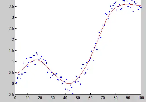
A kernel smoother is a statistical technique to estimate a real valued function as the weighted average of neighboring observed data. The weight is defined by the kernel, such that closer points are given higher weights. The estimated function is smooth, and the level of smoothness is set by a single parameter.
This technique is most appropriate when the dimension of the predictor is low (p < 3), for example for data visualization.
Definitions
Let be a kernel defined by
where:
- is the Euclidean norm
- is a parameter (kernel radius)
- D(t) is typically a positive real valued function, whose value is decreasing (or not increasing) for the increasing distance between the X and X0.
Popular kernels used for smoothing include parabolic (Epanechnikov), Tricube, and Gaussian kernels.
Let be a continuous function of X. For each , the Nadaraya-Watson kernel-weighted average (smooth Y(X) estimation) is defined by
where:
- N is the number of observed points
- Y(Xi) are the observations at Xi points.
In the following sections, we describe some particular cases of kernel smoothers.
Gaussian kernel smoother
The Gaussian kernel is one of the most widely used kernels, and is expressed with the equation below.
Here, b is the length scale for the input space.

Nearest neighbor smoother
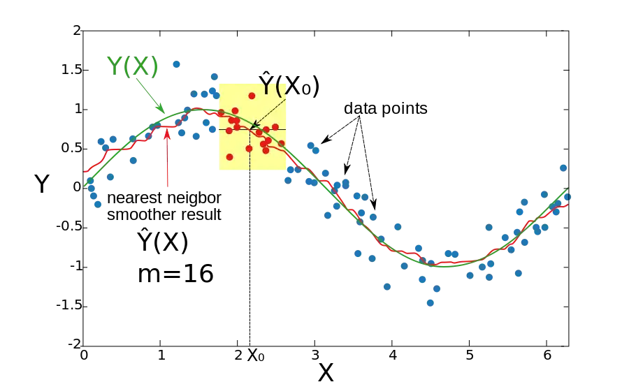
The idea of the nearest neighbor smoother is the following. For each point X0, take m nearest neighbors and estimate the value of Y(X0) by averaging the values of these neighbors.
Formally, , where is the mth closest to X0 neighbor, and
Example:

In this example, X is one-dimensional. For each X0, the is an average value of 16 closest to X0 points (denoted by red). The result is not smooth enough.
Kernel average smoother
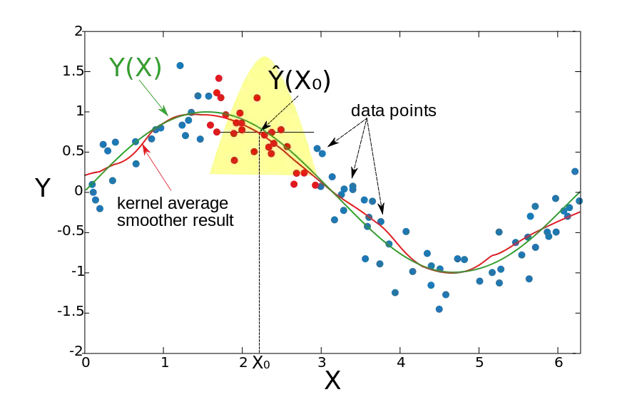
The idea of the kernel average smoother is the following. For each data point X0, choose a constant distance size λ (kernel radius, or window width for p = 1 dimension), and compute a weighted average for all data points that are closer than to X0 (the closer to X0 points get higher weights).
Formally, and D(t) is one of the popular kernels.
Example:

For each X0 the window width is constant, and the weight of each point in the window is schematically denoted by the yellow figure in the graph. It can be seen that the estimation is smooth, but the boundary points are biased. The reason for that is the non-equal number of points (from the right and from the left to the X0) in the window, when the X0 is close enough to the boundary.
Local linear regression
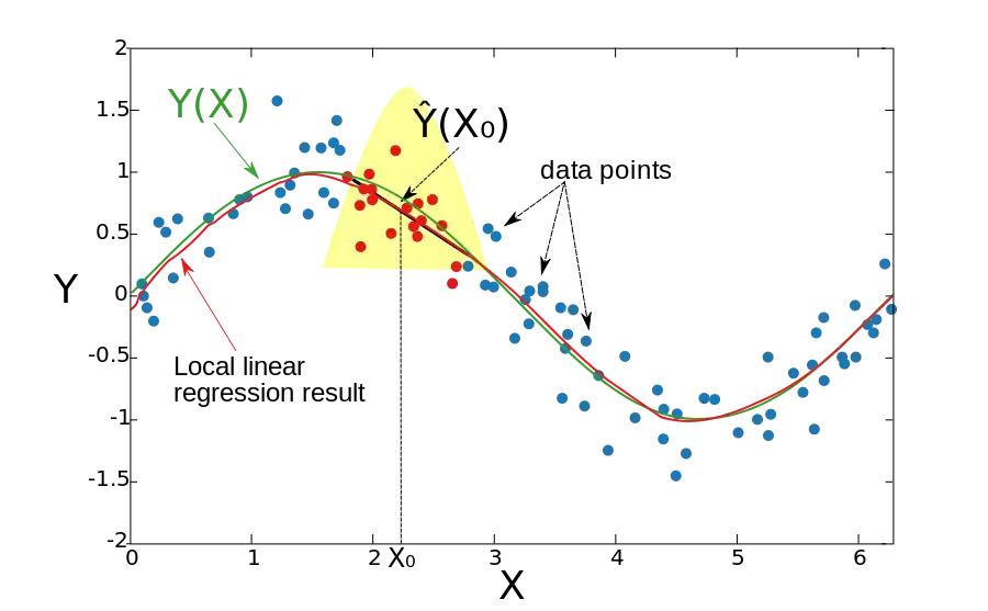
In the two previous sections we assumed that the underlying Y(X) function is locally constant, therefore we were able to use the weighted average for the estimation. The idea of local linear regression is to fit locally a straight line (or a hyperplane for higher dimensions), and not the constant (horizontal line). After fitting the line, the estimation is provided by the value of this line at X0 point. By repeating this procedure for each X0, one can get the estimation function . Like in previous section, the window width is constant Formally, the local linear regression is computed by solving a weighted least square problem.
For one dimension (p = 1):
The closed form solution is given by:
where:
Example:

The resulting function is smooth, and the problem with the biased boundary points is reduced.
Local linear regression can be applied to any-dimensional space, though the question of what is a local neighborhood becomes more complicated. It is common to use k nearest training points to a test point to fit the local linear regression. This can lead to high variance of the fitted function. To bound the variance, the set of training points should contain the test point in their convex hull (see Gupta et al. reference).
Local polynomial regression
Instead of fitting locally linear functions, one can fit polynomial functions.
For p=1, one should minimize:
with
In general case (p>1), one should minimize:
See also
References
- Li, Q. and J.S. Racine. Nonparametric Econometrics: Theory and Practice. Princeton University Press, 2007, ISBN 0-691-12161-3.
- T. Hastie, R. Tibshirani and J. Friedman, The Elements of Statistical Learning, Chapter 6, Springer, 2001. ISBN 0-387-95284-5 (companion book site).
- M. Gupta, E. Garcia and E. Chin, "Adaptive Local Linear Regression with Application to Printer Color Management," IEEE Trans. Image Processing 2008.
