Linear dynamical system
Linear dynamical systems are dynamical systems whose evaluation functions are linear. While dynamical systems, in general, do not have closed-form solutions, linear dynamical systems can be solved exactly, and they have a rich set of mathematical properties. Linear systems can also be used to understand the qualitative behavior of general dynamical systems, by calculating the equilibrium points of the system and approximating it as a linear system around each such point.
Introduction
In a linear dynamical system, the variation of a state vector (an -dimensional vector denoted ) equals a constant matrix (denoted ) multiplied by . This variation can take two forms: either as a flow, in which varies continuously with time
or as a mapping, in which varies in discrete steps
These equations are linear in the following sense: if and are two valid solutions, then so is any linear combination of the two solutions, e.g., where and are any two scalars. The matrix need not be symmetric.
Linear dynamical systems can be solved exactly, in contrast to most nonlinear ones. Occasionally, a nonlinear system can be solved exactly by a change of variables to a linear system. Moreover, the solutions of (almost) any nonlinear system can be well-approximated by an equivalent linear system near its fixed points. Hence, understanding linear systems and their solutions is a crucial first step to understanding the more complex nonlinear systems.
Solution of linear dynamical systems
If the initial vector is aligned with a right eigenvector of the matrix , the dynamics are simple
where is the corresponding eigenvalue; the solution of this equation is
as may be confirmed by substitution.
If is diagonalizable, then any vector in an -dimensional space can be represented by a linear combination of the right and left eigenvectors (denoted ) of the matrix .
Therefore, the general solution for is a linear combination of the individual solutions for the right eigenvectors
Similar considerations apply to the discrete mappings.
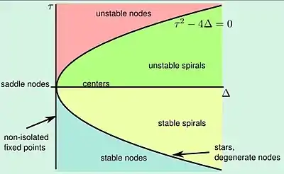
Classification in two dimensions

The roots of the characteristic polynomial det(A - λI) are the eigenvalues of A. The sign and relation of these roots, , to each other may be used to determine the stability of the dynamical system
For a 2-dimensional system, the characteristic polynomial is of the form where is the trace and is the determinant of A. Thus the two roots are in the form:
- ,
and and . Thus if then the eigenvalues are of opposite sign, and the fixed point is a saddle. If then the eigenvalues are of the same sign. Therefore, if both are positive and the point is unstable, and if then both are negative and the point is stable. The discriminant will tell you if the point is nodal or spiral (i.e. if the eigenvalues are real or complex).
