Multilinear subspace learning
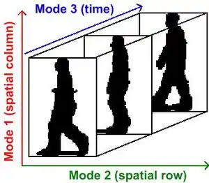
Multilinear subspace learning is an approach to dimensionality reduction.[1][2][3][4][5] Dimensionality reduction can be performed on a data tensor whose observations have been vectorized[1] and organized into a data tensor, or whose observations are matrices that are concatenated into a data tensor.[6][7] Here are some examples of data tensors whose observations are vectorized or whose observations are matrices concatenated into data tensor images (2D/3D), video sequences (3D/4D), and hyperspectral cubes (3D/4D).

The mapping from a high-dimensional vector space to a set of lower dimensional vector spaces is a multilinear projection.[4] When observations are retained in the same organizational structure as the sensor provides them; as matrices or higher order tensors, their representations are computed by performing N multiple linear projections.[6]
Multilinear subspace learning algorithms are higher-order generalizations of linear subspace learning methods such as principal component analysis (PCA), independent component analysis (ICA), linear discriminant analysis (LDA) and canonical correlation analysis (CCA).
Background
With the advances in data acquisition and storage technology, big data (or massive data sets) are being generated on a daily basis in a wide range of emerging applications. Most of these big data are multidimensional. Moreover, they are usually very-high-dimensional, with a large amount of redundancy, and only occupying a part of the input space. Therefore, dimensionality reduction is frequently employed to map high-dimensional data to a low-dimensional space while retaining as much information as possible.
Linear subspace learning algorithms are traditional dimensionality reduction techniques that represent input data as vectors and solve for an optimal linear mapping to a lower-dimensional space. Unfortunately, they often become inadequate when dealing with massive multidimensional data. They result in very-high-dimensional vectors, lead to the estimation of a large number of parameters.[1][6][7][8][9]
Multilinear Subspace Learning employ different types of data tensor analysis tools for dimensionality reduction. Multilinear Subspace learning can be applied to observations whose measurements were vectorized and organized into a data tensor,[1] or whose measurements are treated as a matrix and concatenated into a tensor.[10]
Algorithms
Multilinear principal component analysis
Historically, multilinear principal component analysis has been referred to as "M-mode PCA", a terminology which was coined by Peter Kroonenberg.[11] In 2005, Vasilescu and Terzopoulos introduced the Multilinear PCA[12] terminology as a way to better differentiate between multilinear tensor decompositions that computed 2nd order statistics associated with each data tensor mode(axis)s,[1][2][3][13][8]and subsequent work on Multilinear Independent Component Analysis[12] that computed higher order statistics associated with each tensor mode/axis. MPCA is an extension of PCA.
Multilinear independent component analysis
Multilinear independent component analysis[12] is an extension of ICA.
Multilinear linear discriminant analysis
Multilinear canonical correlation analysis
- Multilinear extension of CCA
- A TTP is a direct projection of a high-dimensional tensor to a low-dimensional tensor of the same order, using N projection matrices for an Nth-order tensor. It can be performed in N steps with each step performing a tensor-matrix multiplication (product). The N steps are exchangeable.[19] This projection is an extension of the higher-order singular value decomposition[19] (HOSVD) to subspace learning.[8] Hence, its origin is traced back to the Tucker decomposition[20] in 1960s.
- A TVP is a direct projection of a high-dimensional tensor to a low-dimensional vector, which is also referred to as the rank-one projections. As TVP projects a tensor to a vector, it can be viewed as multiple projections from a tensor to a scalar. Thus, the TVP of a tensor to a P-dimensional vector consists of P projections from the tensor to a scalar. The projection from a tensor to a scalar is an elementary multilinear projection (EMP). In EMP, a tensor is projected to a point through N unit projection vectors. It is the projection of a tensor on a single line (resulting a scalar), with one projection vector in each mode. Thus, the TVP of a tensor object to a vector in a P-dimensional vector space consists of P EMPs. This projection is an extension of the canonical decomposition,[21] also known as the parallel factors (PARAFAC) decomposition.[22]
Typical approach in MSL
There are N sets of parameters to be solved, one in each mode. The solution to one set often depends on the other sets (except when N=1, the linear case). Therefore, the suboptimal iterative procedure in[23] is followed.
- Initialization of the projections in each mode
- For each mode, fixing the projection in all the other mode, and solve for the projection in the current mode.
- Do the mode-wise optimization for a few iterations or until convergence.
This is originated from the alternating least square method for multi-way data analysis.[11]
Pros and cons

The advantages of MSL over traditional linear subspace modeling, in common domains where the representation is naturally somewhat tensorial, are:[6][7][8][9]
- MSL preserves the structure and correlation that the original data had before projection, by operating on a natural tensorial representation of the multidimensional data.
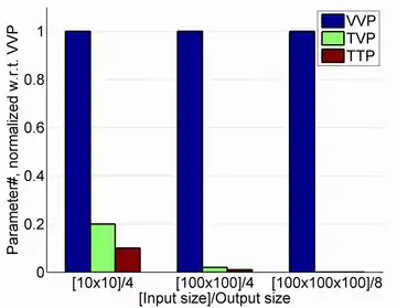
- MSL can learn more compact representations than its linear counterpart; in other words, it needs to estimate a much smaller number of parameters. Thus, MSL can handle big tensor data more efficiently, by performing computations on a representation with many fewer dimensions. This leads to lower demand on computational resources.
However, MSL algorithms are iterative and are not guaranteed to converge; where an MSL algorithm does converge, it may do so at a local optimum. (In contrast, traditional linear subspace modeling techniques often produce an exact closed-form solution.) MSL convergence problems can often be mitigated by choosing an appropriate subspace dimensionality, and by appropriate strategies for initialization, for termination, and for choosing the order in which projections are solved.[6][7][8][9]
Pedagogical resources
- Survey: A survey of multilinear subspace learning for tensor data (open access version).
- Lecture: Video lecture on UMPCA at the 25th International Conference on Machine Learning (ICML 2008).
Code
Tensor data sets
- 3D gait data (third-order tensors): 128x88x20(21.2M); 64x44x20(9.9M); 32x22x10(3.2M);
See also
References
- M. A. O. Vasilescu, D. Terzopoulos (2003) "Multilinear Subspace Analysis of Image Ensembles", "Proceedings of the IEEE Conference on Computer Vision and Pattern Recognition (CVPR’03), Madison, WI, June, 2003"
- M. A. O. Vasilescu, D. Terzopoulos (2002) "Multilinear Analysis of Image Ensembles: TensorFaces", Proc. 7th European Conference on Computer Vision (ECCV'02), Copenhagen, Denmark, May, 2002
- M. A. O. Vasilescu,(2002) "Human Motion Signatures: Analysis, Synthesis, Recognition", "Proceedings of International Conference on Pattern Recognition (ICPR 2002), Vol. 3, Quebec City, Canada, Aug, 2002, 456–460."
- Vasilescu, M.A.O.; Terzopoulos, D. (2007). Multilinear Projection for Appearance-Based Recognition in the Tensor Framework. IEEE 11th International Conference on Computer Vision. pp. 1–8. doi:10.1109/ICCV.2007.4409067..
- Lu, Haiping; Plataniotis, K.N.; Venetsanopoulos, A.N. (2013). Multilinear Subspace Learning: Dimensionality Reduction of Multidimensional Data. Chapman & Hall/CRC Press Machine Learning and Pattern Recognition Series. Taylor and Francis. ISBN 978-1-4398572-4-3.
- Lu, Haiping; Plataniotis, K.N.; Venetsanopoulos, A.N. (2011). "A Survey of Multilinear Subspace Learning for Tensor Data" (PDF). Pattern Recognition. 44 (7): 1540–1551. doi:10.1016/j.patcog.2011.01.004.
- X. He, D. Cai, P. Niyogi, Tensor subspace analysis, in: Advances in Neural Information Processing Systemsc 18 (NIPS), 2005.
- H. Lu, K. N. Plataniotis, and A. N. Venetsanopoulos, "MPCA: Multilinear principal component analysis of tensor objects," IEEE Trans. Neural Netw., vol. 19, no. 1, pp. 18–39, January 2008.
- S. Yan, D. Xu, Q. Yang, L. Zhang, X. Tang, and H.-J. Zhang, "Discriminant analysis with tensor representation," in Proc. IEEE Conference on Computer Vision and Pattern Recognition, vol. I, June 2005, pp. 526–532.
- "Future Directions in Tensor-Based Computation and Modeling" (PDF). May 2009.
- P. M. Kroonenberg and J. de Leeuw, Principal component analysis of three-mode data by means of alternating least squares algorithms, Psychometrika, 45 (1980), pp. 69–97.
- M. A. O. Vasilescu, D. Terzopoulos (2005) "Multilinear Independent Component Analysis", "Proceedings of the IEEE Conference on Computer Vision and Pattern Recognition (CVPR’05), San Diego, CA, June 2005, vol.1, 547–553."
- M.A.O. Vasilescu, D. Terzopoulos (2004) "TensorTextures: Multilinear Image-Based Rendering", M. A. O. Vasilescu and D. Terzopoulos, Proc. ACM SIGGRAPH 2004 Conference Los Angeles, CA, August, 2004, in Computer Graphics Proceedings, Annual Conference Series, 2004, 336–342.
- D. Tao, X. Li, X. Wu, and S. J. Maybank, "General tensor discriminant analysis and gabor features for gait recognition," IEEE Trans. Pattern Anal. Mach. Intell., vol. 29, no. 10, pp. 1700–1715, October 2007.
- H. Lu, K. N. Plataniotis, and A. N. Venetsanopoulos, "Uncorrelated multilinear discriminant analysis with regularization and aggregation for tensor object recognition," IEEE Trans. Neural Netw., vol. 20, no. 1, pp. 103–123, January 2009.
- T.-K. Kim and R. Cipolla. "Canonical correlation analysis of video volume tensors for action categorization and detection," IEEE Trans. Pattern Anal. Mach. Intell., vol. 31, no. 8, pp. 1415–1428, 2009.
- H. Lu, "Learning Canonical Correlations of Paired Tensor Sets via Tensor-to-Vector Projection," Proceedings of the 23rd International Joint Conference on Artificial Intelligence (IJCAI 2013), Beijing, China, August 3–9, 2013.
- Khan, Suleiman A.; Kaski, Samuel (2014-09-15). Calders, Toon; Esposito, Floriana; Hüllermeier, Eyke; Meo, Rosa (eds.). Machine Learning and Knowledge Discovery in Databases. Lecture Notes in Computer Science. Springer Berlin Heidelberg. pp. 656–671. doi:10.1007/978-3-662-44848-9_42. ISBN 9783662448472.
- L.D. Lathauwer, B.D. Moor, J. Vandewalle, A multilinear singular value decomposition, SIAM Journal of Matrix Analysis and Applications vol. 21, no. 4, pp. 1253–1278, 2000
- Ledyard R Tucker (September 1966). "Some mathematical notes on three-mode factor analysis". Psychometrika. 31 (3): 279–311. doi:10.1007/BF02289464. PMID 5221127.
- J. D. Carroll & J. Chang (1970). "Analysis of individual differences in multidimensional scaling via an n-way generalization of 'Eckart–Young' decomposition". Psychometrika. 35 (3): 283–319. doi:10.1007/BF02310791.
- R. A. Harshman, Foundations of the PARAFAC procedure: Models and conditions for an "explanatory" multi-modal factor analysis Archived 2004-10-10 at the Wayback Machine. UCLA Working Papers in Phonetics, 16, pp. 1–84, 1970.
- L. D. Lathauwer, B. D. Moor, J. Vandewalle, On the best rank-1 and rank-(R1, R2, ..., RN ) approximation of higher-order tensors, SIAM Journal of Matrix Analysis and Applications 21 (4) (2000) 1324–1342.
