Time-activity curve
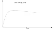
In medical imaging, a time-activity curve is a curve of radioactivity (in terms of concentration) plotted on the y-axis against the time plotted on the x-axis. It shows the concentration of a radiotracer within a region of interest in an image, measured over time from a dynamic scan. Generally, when a time-activity curve is obtained within a tissue, it is called as a tissue time-activity curve, which represents the concentration of tracer within a region of interest inside a tissue over time.

Modern kinetic analysis is performed in various medical imaging techniques, which requires a tissue time-activity curve as one of the inputs to the mathematical model, for example, in dynamic positron emission tomography (PET) imaging, or perfusion CT, or dynamic contrast-enhanced magnetic resonance imaging (DCE-MRI) using a dynamic scan. A dynamic scan is a scan where two dimensional (2D) or three dimensional (3D) images are acquired again and again over a time-period forming a time-series of 2D/3D image datasets. For example, a dynamic contrast-enhanced magnetic resonance imaging scan acquired over ten minutes contains short image frames acquired for 30 seconds duration to capture the fast dynamics of gadolinium tracer. Each data-point in the time-activity curve represents a measurement of tracer-concentration from the region segmented on each of these image time-frame acquired over time.
Obtaining the time-activity curve
Time-activity curves are obtained with the help of region-of-interest analysis. The region-of-interest analysis restricts the image data to a specific region on which measurements can be made, for example, lumbar vertebrae or the femoral neck. The image pixels within that specifically marked region is then replicated on all of the image frames of the dynamic scan, and an average pixel value from all image-frames is then plotted against the time at which these image-frames were obtained.
The concept is explained with an example below. Consider a dynamic image where each table represents an image, obtained at different times, let's say at time t=1 sec, t=2 sec, t=3 sec, t=4 sec, t=5 sec, and t=6 sec. In this image, let's assume, each voxel shows the concentration of tracer in the units Bq per ml. Now, let's say our target region within each image is only the central four voxels. First, the central four pixels in each image are identified, which is our region-of-interest, then an average is taken for each frame.
|
|
|
|
|
|
|---|
t=1 sec........... t=2 sec............t=3 sec............t=4 sec............t=5 sec............t=6 sec
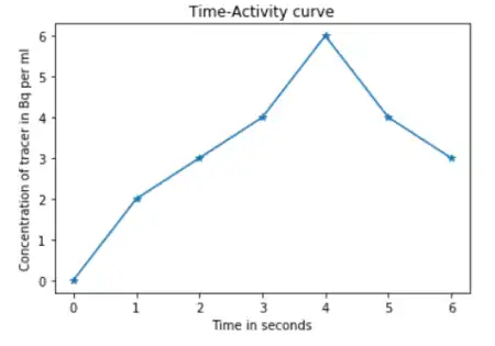
In this example, we would have an average value of 2 for the 1st frame at t=1, 3 for the 2nd frame at t=2, 4 for the 3rd frame at t=3, 6 for the 4th frame at t=4, 4 for the 5th frame at t=5, and 3 for the 6th frame at t=6. Now, these values can be plotted on a graph, where time is on the x-axis, and the averaged concentration values on the y-axis. The graph will look like as follows (assuming that pixel values in the image will be 0 at t=0):

The region of interest (the central four pixels in the above examples) can be identified using manual,[1] semi-automatic,[2] or automatic[3] methods. The manual region of interest definition requires the user to draw an arbitrary boundary around the target region, which is subjective. The boundary can be marked by points or lines with different thickness levels. The selection can also be achieved by choosing the co-ordinate values. When selecting a region of interest the user can keep track of the properties of the boundary pixels, for example, the position and the value of the currently selected pixel.
Semi-automatic methods define a region of interest with minimum user interaction, and can be broadly classified into geometric selection,[4][2] thresholding,[5] and region growing methods,[6] or a combination of any two or any other criteria.[7] In thresholding methods, pixels above a certain intensity level in an image are included in the region of interest. In region growing methods, a user selects a seed pixel that identifies the first pixel within the region of interest and based on a stopping criterion the neighbouring pixels are attached to the seed pixel and when the algorithm stops the pixels surrounding the seed pixels form a region of interest.
Automatic methods do not require user intervention,[8] and are also referred to as iterative or adaptive methods, as they work based on prior knowledge of the region to be analysed. The majority of the semi-automatic methods can also be automated but they do need to be validated against the manual gold-standard drawn by experts.[2][9]
Relationship with the arterial input function
Obtaining the time-activity curve within an artery is the first towards obtaining the image-derived arterial input function (IDAIF). The arterial time-activity curve is then corrected for various errors using arterial/venous blood-sample before an arterial input function (AIF) can be used as an input to the model for kinetic analysis.
References
- Mykkänen, Jouni M.; Juhola, Martti; Ruotsalainen, Ulla (2000). "Extracting VOIs from brain PET images". International Journal of Medical Informatics. 58-59: 51–57. doi:10.1016/s1386-5056(00)00075-7. ISSN 1386-5056.
- Puri, T.; Blake, G. M.; Curran, K. M.; Carr, H.; Moore, A. E. B.; Colgan, N.; O'Connell, M. J.; Marsden, P. K.; Fogelman, I.; Frost, M. L. (2012). "Semi-automatic Region-of-Interest Validation at the Femur in 18F-Fluoride PET/CT". Journal of Nuclear Medicine Technology. 40 (3): 168–174. doi:10.2967/jnmt.111.100107. ISSN 0091-4916.
- Feng, Yue; Fang, Hui; Jiang, Jianmin (2005), "Region Growing with Automatic Seeding for Semantic Video Object Segmentation", Pattern Recognition and Image Analysis, Springer Berlin Heidelberg, pp. 542–549, ISBN 978-3-540-28833-6, retrieved 2020 Check date values in:
|access-date=(help) - Krak, Nanda C.; Boellaard, R.; Hoekstra, Otto S.; Twisk, Jos W. R.; Hoekstra, Corneline J.; Lammertsma, Adriaan A. (2004). "Effects of ROI definition and reconstruction method on quantitative outcome and applicability in a response monitoring trial". European Journal of Nuclear Medicine and Molecular Imaging. 32 (3): 294–301. doi:10.1007/s00259-004-1566-1. ISSN 1619-7070.
- Sankur, Bu¨lent (2004). "Survey over image thresholding techniques and quantitative performance evaluation". Journal of Electronic Imaging. 13 (1): 146. doi:10.1117/1.1631315. ISSN 1017-9909.
- ZHENG, L., JESSE, J. & HUGUES, T. (2001) Unseeded region growing for 3D image segmentation. Selected papers from the Pan-Sydney workshop on Visualisation – Volume 2. Sydney, Australia, Australian Computer Society, Inc.
- Pan, Zhigeng; Lu, Jianfeng (2007). "A Bayes-Based Region-Growing Algorithm for Medical Image Segmentation". Computing in Science & Engineering. 9 (4): 32–38. doi:10.1109/mcse.2007.67. ISSN 1521-9615.
- Suzuki, H.; Toriwaki, J. "Knowledge-guided automatic thresholding for 3-dimensional display of head MRI images". [1988 Proceedings] 9th International Conference on Pattern Recognition. IEEE Comput. Soc. Press. doi:10.1109/icpr.1988.28473. ISBN 0-8186-0878-1.
- Weaver, Jean R.; Au, Jessie L-S. (1 October 1997). <128::aid-cyto5>3.0.co;2-9 "Application of automatic thresholding in image analysis scoring of cells in human solid tumors labeled for proliferation markers". Cytometry. 29 (2): 128–135. doi:10.1002/(sici)1097-0320(19971001)29:2<128::aid-cyto5>3.0.co;2-9. ISSN 0196-4763.