Viterbi algorithm

The Viterbi algorithm is named after Andrew Viterbi, who proposed it in 1967 as a decoding algorithm for convolutional codes over noisy digital communication links.[2] It has, however, a history of multiple invention, with at least seven independent discoveries, including those by Viterbi, Needleman and Wunsch, and Wagner and Fischer.[3] It was introduced to Natural Language Processing as a method of Part-of-speech tagging as early as 1987.

"Viterbi path" and "Viterbi algorithm" have become standard terms for the application of dynamic programming algorithms to maximization problems involving probabilities.[3] For example, in statistical parsing a dynamic programming algorithm can be used to discover the single most likely context-free derivation (parse) of a string, which is commonly called the "Viterbi parse".[4][5][6] Another application is in target tracking, where the track is computed that assigns a maximum likelihood to a sequence of observations.[7]

A generalization of the Viterbi algorithm, termed the max-sum algorithm (or max-product algorithm) can be used to find the most likely assignment of all or some subset of latent variables in a large number of graphical models, e.g. Bayesian networks, Markov random fields and conditional random fields. The latent variables need in general to be connected in a way somewhat similar to an HMM, with a limited number of connections between variables and some type of linear structure among the variables. The general algorithm involves message passing and is substantially similar to the belief propagation algorithm (which is the generalization of the forward-backward algorithm).

With the algorithm called iterative Viterbi decoding one can find the subsequence of an observation that matches best (on average) to a given hidden Markov model. This algorithm is proposed by Qi Wang et al. to deal with turbo code.[8] Iterative Viterbi decoding works by iteratively invoking a modified Viterbi algorithm, reestimating the score for a filler until convergence.

An alternative algorithm, the Lazy Viterbi algorithm, has been proposed.[9] For many applications of practical interest, under reasonable noise conditions, the lazy decoder (using Lazy Viterbi algorithm) is much faster than the original Viterbi decoder (using Viterbi algorithm). While the original Viterbi algorithm calculates every node in the trellis of possible outcomes, the Lazy Viterbi algorithm maintains a prioritized list of nodes to evaluate in order, and the number of calculations required is typically fewer (and never more) than the ordinary Viterbi algorithm for the same result. However, it is not so easy to parallelize in hardware.

This algorithm generates a path ${\displaystyle X=(x_{1},x_{2},\ldots ,x_{T})}$, which is a sequence of states ${\displaystyle x_{n}\in S=\{s_{1},s_{2},\dots ,s_{K}\}}$ that generate the observations ${\displaystyle Y=(y_{1},y_{2},\ldots ,y_{T})}$ with ${\displaystyle y_{n}\in O=\{o_{1},o_{2},\dots ,o_{N}\}}$, where ${\displaystyle N}$ is the number of possible observations in the observation space ${\displaystyle O}$.

Two 2-dimensional tables of size ${\displaystyle K\times T}$ are constructed:

• Each element ${\displaystyle T_{1}[i,j]}$ of ${\displaystyle T_{1}}$ stores the probability of the most likely path so far ${\displaystyle {\hat {X}}=({\hat {x}}_{1},{\hat {x}}_{2},\ldots ,{\hat {x}}_{j})}$ with ${\displaystyle {\hat {x}}_{j}=s_{i}}$ that generates ${\displaystyle Y=(y_{1},y_{2},\ldots ,y_{j})}$.
• Each element ${\displaystyle T_{2}[i,j]}$ of ${\displaystyle T_{2}}$ stores ${\displaystyle {\hat {x}}_{j-1}}$ of the most likely path so far ${\displaystyle {\hat {X}}=({\hat {x}}_{1},{\hat {x}}_{2},\ldots ,{\hat {x}}_{j-1},{\hat {x}}_{j}=s_{i})}$ for ${\displaystyle \forall j,2\leq j\leq T}$

The table entries ${\displaystyle T_{1}[i,j],T_{2}[i,j]}$ are filled by increasing order of ${\displaystyle K\cdot j+i}$:

${\displaystyle T_{1}[i,j]=\max _{k}{(T_{1}[k,j-1]\cdot A_{ki}\cdot B_{iy_{j}})}}$,

${\displaystyle T_{2}[i,j]=\operatorname {argmax} _{k}{(T_{1}[k,j-1]\cdot A_{ki}\cdot B_{iy_{j}})}}$,

with ${\displaystyle A_{ki}}$ and ${\displaystyle B_{iy_{j}}}$ as defined below. Note that ${\displaystyle B_{iy_{j}}}$ does not need to appear in the latter expression, as it's non-negative and independent of ${\displaystyle k}$ and thus does not affect the argmax.

Input

• The observation space ${\displaystyle O=\{o_{1},o_{2},\dots ,o_{N}\}}$,
• the state space ${\displaystyle S=\{s_{1},s_{2},\dots ,s_{K}\}}$,
• an array of initial probabilities ${\displaystyle \Pi =(\pi _{1},\pi _{2},\dots ,\pi _{K})}$ such that ${\displaystyle \pi _{i}}$ stores the probability that ${\displaystyle x_{1}=s_{i}}$,
• a sequence of observations ${\displaystyle Y=(y_{1},y_{2},\ldots ,y_{T})}$ such that ${\displaystyle y_{t}=i}$ if the observation at time ${\displaystyle t}$ is ${\displaystyle o_{i}}$,
• transition matrix ${\displaystyle A}$ of size ${\displaystyle K\times K}$ such that ${\displaystyle A_{ij}}$ stores the transition probability of transiting from state ${\displaystyle s_{i}}$ to state ${\displaystyle s_{j}}$,
• emission matrix ${\displaystyle B}$ of size ${\displaystyle K\times N}$ such that ${\displaystyle B_{ij}}$ stores the probability of observing ${\displaystyle o_{j}}$ from state ${\displaystyle s_{i}}$.

Output

• The most likely hidden state sequence ${\displaystyle X=(x_{1},x_{2},\ldots ,x_{T})}$

function VITERBI${\displaystyle (O,S,\Pi ,Y,A,B):X}$
    for each state ${\displaystyle i=1,2,\ldots ,K}$ do
        ${\displaystyle T_{1}[i,1]\leftarrow \pi _{i}\cdot B_{iy_{1}}}$
        ${\displaystyle T_{2}[i,1]\leftarrow 0}$
    end for
    for each observation ${\displaystyle j=2,3,\ldots ,T}$ do
        for each state ${\displaystyle i=1,2,\ldots ,K}$ do
            ${\displaystyle T_{1}[i,j]\gets \max _{k}{(T_{1}[k,j-1]\cdot A_{ki}\cdot B_{iy_{j}})}}$
            ${\displaystyle T_{2}[i,j]\gets \arg \max _{k}{(T_{1}[k,j-1]\cdot A_{ki}\cdot B_{iy_{j}})}}$
        end for
    end for
    ${\displaystyle z_{T}\gets \arg \max _{k}{(T_{1}[k,T])}}$
    ${\displaystyle x_{T}\leftarrow s_{z_{T}}}$
    for ${\displaystyle j=T,T-1,\ldots ,2}$ do
        ${\displaystyle z_{j-1}\leftarrow T_{2}[z_{j},j]}$
        ${\displaystyle x_{j-1}\leftarrow s_{z_{j-1}}}$
    end for
    return ${\displaystyle X}$
end function

Restated in a succinct near-Python:

# probability == p. Tm: the transition matrix. Em: the emission matrix.
function viterbi(O, S, Π, Tm, Em): best_path 
    trellis ← matrix(length(S), length(O))  # To hold p. of each state given each observation.
    # Determine each hidden state's p. at time 0…
    for s in range(length(S)):
        trellis[s, 0] ← Π[s] * Em[s, O[0]] 
    # …and afterwards, assuming each state's most likely prior state, k.
    for o in range(1, length(O)):
        for s in range(length(S)):
            k ← argmax(k in trellis[k, o-1] * Tm[k, s] * Em[s, o])
            trellis[s, o] ← trellis[k, o-1] * Tm[k, s] * Em[s, o]
    best_path ← list()
    for o in range(-1, -(length(O)+1), -1):  # Backtrack from last observation.
        k ← argmax(k in trellis[k, o])  # Most likely state at o 
        best_path.insert(0, S[k])       # is noted for return.
    return best_path

Explanation

Suppose we are given a hidden Markov model (HMM) with state space ${\displaystyle S}$, initial probabilities ${\displaystyle \pi _{i}}$ of being in state ${\displaystyle i}$ and transition probabilities ${\displaystyle a_{i,j}}$ of transitioning from state ${\displaystyle i}$ to state ${\displaystyle j}$. Say, we observe outputs ${\displaystyle y_{1},\dots ,y_{T}}$. The most likely state sequence ${\displaystyle x_{1},\dots ,x_{T}}$ that produces the observations is given by the recurrence relations[10]

${\displaystyle {\begin{aligned}V_{1,k}&=\mathrm {P} {\big (}y_{1}\ |\ k{\big )}\cdot \pi _{k},\\V_{t,k}&=\max _{x\in S}\left(\mathrm {P} {\big (}y_{t}\ |\ k{\big )}\cdot a_{x,k}\cdot V_{t-1,x}\right).\end{aligned}}}$

Here ${\displaystyle V_{t,k}}$ is the probability of the most probable state sequence ${\displaystyle \mathrm {P} {\big (}x_{1},\dots ,x_{t},y_{1},\dots ,y_{t}{\big )}}$ responsible for the first ${\displaystyle t}$ observations that have ${\displaystyle k}$ as its final state. The Viterbi path can be retrieved by saving back pointers that remember which state ${\displaystyle x}$ was used in the second equation. Let ${\displaystyle \mathrm {Ptr} (k,t)}$ be the function that returns the value of ${\displaystyle x}$ used to compute ${\displaystyle V_{t,k}}$ if ${\displaystyle t>1}$, or ${\displaystyle k}$ if ${\displaystyle t=1}$. Then

${\displaystyle {\begin{aligned}x_{T}&=\arg \max _{x\in S}(V_{T,x}),\\x_{t-1}&=\mathrm {Ptr} (x_{t},t).\end{aligned}}}$

Here we're using the standard definition of arg max.

The complexity of this implementation is ${\displaystyle O(T\times \left|{S}\right|^{2})}$. A better estimation exists if the maximum in the internal loop is instead found by iterating only over states that directly link to the current state (i.e. there is an edge from ${\displaystyle k}$ to ${\displaystyle j}$). Then using amortized analysis one can show that the complexity is ${\displaystyle O(T\times (\left|{S}\right|+\left|{E}\right|))}$, where ${\displaystyle E}$ is the number of edges in the graph.

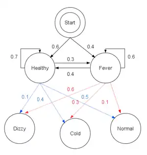
Consider a village where all villagers are either healthy or have a fever and only the village doctor can determine whether each has a fever. The doctor diagnoses fever by asking patients how they feel. The villagers may only answer that they feel normal, dizzy, or cold.

The doctor believes that the health condition of his patients operates as a discrete Markov chain. There are two states, "Healthy" and "Fever", but the doctor cannot observe them directly; they are hidden from him. On each day, there is a certain chance that the patient will tell the doctor he is "normal", "cold", or "dizzy", depending on their health condition.

The observations (normal, cold, dizzy) along with a hidden state (healthy, fever) form a hidden Markov model (HMM), and can be represented as follows in the Python programming language:

obs = ("normal", "cold", "dizzy")
states = ("Healthy", "Fever")
start_p = {"Healthy": 0.6, "Fever": 0.4}
trans_p = {
    "Healthy": {"Healthy": 0.7, "Fever": 0.3},
    "Fever": {"Healthy": 0.4, "Fever": 0.6},
}
emit_p = {
    "Healthy": {"normal": 0.5, "cold": 0.4, "dizzy": 0.1},
    "Fever": {"normal": 0.1, "cold": 0.3, "dizzy": 0.6},
}

In this piece of code, start_p represents the doctor's belief about which state the HMM is in when the patient first visits (all he knows is that the patient tends to be healthy). The particular probability distribution used here is not the equilibrium one, which is (given the transition probabilities) approximately {'Healthy': 0.57, 'Fever': 0.43}. The transition_p represents the change of the health condition in the underlying Markov chain. In this example, there is only a 30% chance that tomorrow the patient will have a fever if he is healthy today. The emission_p represents how likely each possible observation, normal, cold, or dizzy is given their underlying condition, healthy or fever. If the patient is healthy, there is a 50% chance that he feels normal; if he has a fever, there is a 60% chance that he feels dizzy.

Graphical representation of the given HMM

The patient visits three days in a row and the doctor discovers that on the first day he feels normal, on the second day he feels cold, on the third day he feels dizzy. The doctor has a question: what is the most likely sequence of health conditions of the patient that would explain these observations? This is answered by the Viterbi algorithm.

def viterbi(obs, states, start_p, trans_p, emit_p):
    V = [{}]
    for st in states:
        V[0][st] = {"prob": start_p[st] * emit_p[st][obs[0]], "prev": None}
    # Run Viterbi when t > 0
    for t in range(1, len(obs)):
        V.append({})
        for st in states:
            max_tr_prob = V[t - 1][states[0]]["prob"] * trans_p[states[0]][st]
            prev_st_selected = states[0]
            for prev_st in states[1:]:
                tr_prob = V[t - 1][prev_st]["prob"] * trans_p[prev_st][st]
                if tr_prob > max_tr_prob:
                    max_tr_prob = tr_prob
                    prev_st_selected = prev_st

            max_prob = max_tr_prob * emit_p[st][obs[t]]
            V[t][st] = {"prob": max_prob, "prev": prev_st_selected}

    for line in dptable(V):
        print(line)

    opt = []
    max_prob = 0.0
    best_st = None
    # Get most probable state and its backtrack
    for st, data in V[-1].items():
        if data["prob"] > max_prob:
            max_prob = data["prob"]
            best_st = st
    opt.append(best_st)
    previous = best_st

    # Follow the backtrack till the first observation
    for t in range(len(V) - 2, -1, -1):
        opt.insert(0, V[t + 1][previous]["prev"])
        previous = V[t + 1][previous]["prev"]

    print ("The steps of states are " + " ".join(opt) + " with highest probability of %s" % max_prob)

def dptable(V):
    # Print a table of steps from dictionary
    yield " ".join(("%12d" % i) for i in range(len(V)))
    for state in V[0]:
        yield "%.7s: " % state + " ".join("%.7s" % ("%f" % v[state]["prob"]) for v in V)

The function viterbi takes the following arguments: obs is the sequence of observations, e.g. ['normal', 'cold', 'dizzy']; states is the set of hidden states; start_p is the start probability; trans_p are the transition probabilities; and emit_p are the emission probabilities. For simplicity of code, we assume that the observation sequence obs is non-empty and that trans_p[i][j] and emit_p[i][j] is defined for all states i,j.

In the running example, the forward/Viterbi algorithm is used as follows:

viterbi(obs,
        states,
        start_p,
        trans_p,
        emit_p)

The output of the script is

$ python viterbi_example.py
         0          1          2
Healthy: 0.30000 0.08400 0.00588
Fever: 0.04000 0.02700 0.01512
The steps of states are Healthy Healthy Fever with highest probability of 0.01512

This reveals that the observations ['normal', 'cold', 'dizzy'] were most likely generated by states ['Healthy', 'Healthy', 'Fever']. In other words, given the observed activities, the patient was most likely to have been healthy both on the first day when he felt normal as well as on the second day when he felt cold, and then he contracted a fever the third day.

The operation of Viterbi's algorithm can be visualized by means of a trellis diagram. The Viterbi path is essentially the shortest path through this trellis.

The soft output Viterbi algorithm (SOVA) is a variant of the classical Viterbi algorithm.

SOVA differs from the classical Viterbi algorithm in that it uses a modified path metric which takes into account the a priori probabilities of the input symbols, and produces a soft output indicating the reliability of the decision.

The first step in the SOVA is the selection of the survivor path, passing through one unique node at each time instant, t. Since each node has 2 branches converging at it (with one branch being chosen to form the Survivor Path, and the other being discarded), the difference in the branch metrics (or cost) between the chosen and discarded branches indicate the amount of error in the choice.

This cost is accumulated over the entire sliding window (usually equals at least five constraint lengths), to indicate the soft output measure of reliability of the hard bit decision of the Viterbi algorithm.

• Expectation–maximization algorithm
• Baum–Welch algorithm
• Forward-backward algorithm
• Forward algorithm
• Error-correcting code
• Viterbi decoder
• Hidden Markov model
• Part-of-speech tagging
• A* search algorithm

• Viterbi AJ (April 1967). "Error bounds for convolutional codes and an asymptotically optimum decoding algorithm". IEEE Transactions on Information Theory. 13 (2): 260–269. doi:10.1109/TIT.1967.1054010. (note: the Viterbi decoding algorithm is described in section IV.) Subscription required.
• Feldman J, Abou-Faycal I, Frigo M (2002). A Fast Maximum-Likelihood Decoder for Convolutional Codes. Vehicular Technology Conference. 1. pp. 371–375. CiteSeerX 10.1.1.114.1314. doi:10.1109/VETECF.2002.1040367. ISBN 978-0-7803-7467-6.
• Forney GD (March 1973). "The Viterbi algorithm". Proceedings of the IEEE. 61 (3): 268–278. doi:10.1109/PROC.1973.9030. Subscription required.
• Press, WH; Teukolsky, SA; Vetterling, WT; Flannery, BP (2007). "Section 16.2. Viterbi Decoding". Numerical Recipes: The Art of Scientific Computing (3rd ed.). New York: Cambridge University Press. ISBN 978-0-521-88068-8.
• Rabiner LR (February 1989). "A tutorial on hidden Markov models and selected applications in speech recognition". Proceedings of the IEEE. 77 (2): 257–286. CiteSeerX 10.1.1.381.3454. doi:10.1109/5.18626. (Describes the forward algorithm and Viterbi algorithm for HMMs).
• Shinghal, R. and Godfried T. Toussaint, "Experiments in text recognition with the modified Viterbi algorithm," IEEE Transactions on Pattern Analysis and Machine Intelligence, Vol. PAMI-l, April 1979, pp. 184–193.
• Shinghal, R. and Godfried T. Toussaint, "The sensitivity of the modified Viterbi algorithm to the source statistics," IEEE Transactions on Pattern Analysis and Machine Intelligence, vol. PAMI-2, March 1980, pp. 181–185.

• Mathematica has an implementation as part of its support for stochastic processes
• Susa signal processing framework provides the C++ implementation for Forward error correction codes and channel equalization here.
• C++
• C#
• Java
• Java 8
• Perl
• Prolog
• Haskell
• Go
• SFIHMM includes code for Viterbi decoding.

• Implementations in Java, F#, Clojure, C# on Wikibooks
• Tutorial on convolutional coding with viterbi decoding, by Chip Fleming
• A tutorial for a Hidden Markov Model toolkit (implemented in C) that contains a description of the Viterbi algorithm
• Viterbi algorithm by Dr. Andrew J. Viterbi (scholarpedia.org).

References

- Xavier Anguera et al., "Speaker Diarization: A Review of Recent Research", retrieved 19. August 2010, IEEE TASLP
- 29 Apr 2005, G. David Forney Jr: The Viterbi Algorithm: A Personal History
- Daniel Jurafsky; James H. Martin. Speech and Language Processing. Pearson Education International. p. 246.
- Schmid, Helmut (2004). Efficient parsing of highly ambiguous context-free grammars with bit vectors (PDF). Proc. 20th Int'l Conf. on Computational Linguistics (COLING). doi:10.3115/1220355.1220379.
- Klein, Dan; Manning, Christopher D. (2003). A* parsing: fast exact Viterbi parse selection (PDF). Proc. 2003 Conf. of the North American Chapter of the Association for Computational Linguistics on Human Language Technology (NAACL). pp. 40–47. doi:10.3115/1073445.1073461.
- Stanke, M.; Keller, O.; Gunduz, I.; Hayes, A.; Waack, S.; Morgenstern, B. (2006). "AUGUSTUS: Ab initio prediction of alternative transcripts". Nucleic Acids Research. 34 (Web Server issue): W435–W439. doi:10.1093/nar/gkl200. PMC 1538822. PMID 16845043.
- Quach, T.; Farooq, M. (1994). "Maximum Likelihood Track Formation with the Viterbi Algorithm". Proceedings of 33rd IEEE Conference on Decision and Control. 1. pp. 271–276. doi:10.1109/CDC.1994.410918.CS1 maint: multiple names: authors list (link)
- Qi Wang; Lei Wei; Rodney A. Kennedy (2002). "Iterative Viterbi Decoding, Trellis Shaping, and Multilevel Structure for High-Rate Parity-Concatenated TCM". IEEE Transactions on Communications. 50: 48–55. doi:10.1109/26.975743.
- A fast maximum-likelihood decoder for convolutional codes (PDF). Vehicular Technology Conference. December 2002. pp. 371–375. doi:10.1109/VETECF.2002.1040367.
- Xing E, slide 11.
General references