Autoencoder
An autoencoder is a type of artificial neural network used to learn efficient data codings in an unsupervised manner.[1] The aim of an autoencoder is to learn a representation (encoding) for a set of data, typically for dimensionality reduction, by training the network to ignore signal “noise”. Along with the reduction side, a reconstructing side is learnt, where the autoencoder tries to generate from the reduced encoding a representation as close as possible to its original input, hence its name. Variants exist, aiming to force the learned representations to assume useful properties.[2] Examples are regularized autoencoders (Sparse, Denoising and Contractive), which are effective in learning representations for subsequent classification tasks,[3] and Variational autoencoders, with applications as generative models.[4] Autoencoders are applied to many problems, from facial recognition[5] to acquiring the semantic meaning of words.[6][7]
| Part of a series on |
| Machine learning and data mining |
|---|
Introduction
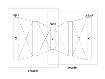
An autoencoder is a neural network that learns to copy its input to its output. It has an internal (hidden) layer that describes a code used to represent the input, and it is constituted by two main parts: an encoder that maps the input into the code, and a decoder that maps the code to a reconstruction of the input.
Performing the copying task perfectly would simply duplicate the signal, and this is why autoencoders usually are restricted in ways that force them to reconstruct the input approximately, preserving only the most relevant aspects of the data in the copy.
The idea of autoencoders has been popular in the field of neural networks for decades. The first applications date to the 1980s.[2][8][9] Their most traditional application was dimensionality reduction or feature learning, but the autoencoder concept became more widely used for learning generative models of data.[10][11] Some of the most powerful AIs in the 2010s involved sparse autoencoders stacked inside deep neural networks.[12]
Basic architecture
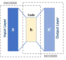
The simplest form of an autoencoder is a feedforward, non-recurrent neural network similar to single layer perceptrons that participate in multilayer perceptrons (MLP) – employing an input layer and an output layer connected by one or more hidden layers. The output layer has the same number of nodes (neurons) as the input layer. Its purpose is to reconstruct its inputs (minimizing the difference between the input and the output) instead of predicting a target value given inputs . Therefore, autoencoders are unsupervised learning models. (They do not require labeled inputs to enable learning).


An autoencoder consists of two parts, the encoder and the decoder, which can be defined as transitions and such that:


In the simplest case, given one hidden layer, the encoder stage of an autoencoder takes the input and maps it to :


This image is usually referred to as code, latent variables, or latent representation. Here, is an element-wise activation function such as a sigmoid function or a rectified linear unit. is a weight matrix and is a bias vector. Weights and biases are usually initialized randomly, and then updated iteratively during training through backpropagation. After that, the decoder stage of the autoencoder maps to the reconstruction of the same shape as :


where for the decoder may be unrelated to the corresponding for the encoder.


Autoencoders are trained to minimise reconstruction errors (such as squared errors), often referred to as the "loss":

where is usually averaged over some input training set.
As mentioned before, the training of an autoencoder is performed through backpropagation of the error, just like a regular feedforward neural network.
Should the feature space have lower dimensionality than the input space , the feature vector can be regarded as a compressed representation of the input . This is the case of undercomplete autoencoders. If the hidden layers are larger than (overcomplete autoencoders), or equal to, the input layer, or the hidden units are given enough capacity, an autoencoder can potentially learn the identity function and become useless. However, experimental results have shown that autoencoders might still learn useful features in these cases.[13] In the ideal setting, one should be able to tailor the code dimension and the model capacity on the basis of the complexity of the data distribution to be modeled. One way to do so is to exploit the model variants known as Regularized Autoencoders.[2]


Variations
Regularized autoencoders
Various techniques exist to prevent autoencoders from learning the identity function and to improve their ability to capture important information and learn richer representations.
Sparse autoencoder (SAE)

When representations are learned in a way that encourages sparsity, improved performance is obtained on classification tasks.[14] Sparse autoencoder may include more (rather than fewer) hidden units than inputs, but only a small number of the hidden units are allowed to be active at the same time.[12] This sparsity constraint forces the model to respond to the unique statistical features of the training data.
Specifically, a sparse autoencoder is an autoencoder whose training criterion involves a sparsity penalty on the code layer .


Recalling that , the penalty encourages the model to activate (i.e. output value close to 1) specific areas of the network on the basis of the input data, while inactivating all other neurons (i.e. to have an output value close to 0).[15]

This sparsity can be achieved by formulating the penalty terms in different ways.
- One way is to exploit the Kullback-Leibler (KL) divergence.[14][15][16][17] Let

be the average activation of the hidden unit (averaged over the training examples). The notation identifies the input value that triggered the activation. To encourage most of the neurons to be inactive, needs to be close to 0. Therefore, this method enforces the constraint where is the sparsity parameter, a value close to zero. The penalty term takes a form that penalizes for deviating significantly from , exploiting the KL divergence:


where is summing over the hidden nodes in the hidden layer, and is the KL-divergence between a Bernoulli random variable with mean and a Bernoulli random variable with mean .[15]


- Another way to achieve sparsity is by applying L1 or L2 regularization terms on the activation, scaled by a certain parameter .[18] For instance, in the case of L1 the loss function becomes


- A further proposed strategy to force sparsity is to manually zero all but the strongest hidden unit activations (k-sparse autoencoder).[19] The k-sparse autoencoder is based on a linear autoencoder (i.e. with linear activation function) and tied weights. The identification of the strongest activations can be achieved by sorting the activities and keeping only the first k values, or by using ReLU hidden units with thresholds that are adaptively adjusted until the k largest activities are identified. This selection acts like the previously mentioned regularization terms in that it prevents the model from reconstructing the input using too many neurons.[19]
Denoising autoencoder (DAE)
Denoising autoencoders (DAE) try to achieve a good representation by changing the reconstruction criterion.[2]
Indeed, DAEs take a partially corrupted input and are trained to recover the original undistorted input. In practice, the objective of denoising autoencoders is that of cleaning the corrupted input, or denoising. Two assumptions are inherent to this approach:
- Higher level representations are relatively stable and robust to the corruption of the input;
- To perform denoising well, the model needs to extract features that capture useful structure in the input distribution.[3]
In other words, denoising is advocated as a training criterion for learning to extract useful features that will constitute better higher level representations of the input.[3]
The training process of a DAE works as follows:
- The initial input is corrupted into through stochastic mapping .
- The corrupted input is then mapped to a hidden representation with the same process of the standard autoencoder, .
- From the hidden representation the model reconstructs .[3]


The model's parameters and are trained to minimize the average reconstruction error over the training data, specifically, minimizing the difference between and the original uncorrupted input .[3] Note that each time a random example is presented to the model, a new corrupted version is generated stochastically on the basis of .


The above-mentioned training process could be applied with any kind of corruption process. Some examples might be additive isotropic Gaussian noise, Masking noise (a fraction of the input chosen at random for each example is forced to 0) or Salt-and-pepper noise (a fraction of the input chosen at random for each example is set to its minimum or maximum value with uniform probability).[3]
The corruption of the input is performed only during training. Once the model has learnt the optimal parameters, in order to extract the representations from the original data no corruption is added.
Contractive autoencoder (CAE)
The contractive autoencoder adds an explicit regularizer in its objective function that forces the model to learn an encoding robust to slight variations of input values. This regularizer corresponds to the Frobenius norm of the Jacobian matrix of the encoder activations with respect to the input. Since the penalty is applied to training examples only, this term forces the model to learn useful information about the training distribution. The final objective function has the following form:

The autoencoder is termed contractive because CAE is encouraged to map a neighborhood of input points to a smaller neighborhood of output points.[2]
DAE is connected to CAE: in the limit of small Gaussian input noise, DAEs make the reconstruction function resist small but finite-sized input perturbations, while CAEs make the extracted features resist infinitesimal input perturbations.
Variational autoencoder (VAE)
Variational autoencoders (VAEs) are generative models, akin to generative adversarial networks.[20] Their association with this group of models derives mainly from the architectural affinity with the basic autoencoder (the final training objective has an encoder and a decoder), but their mathematical formulation differs significantly.[21] VAEs are directed probabilistic graphical models (DPGM) whose posterior is approximated by a neural network, forming an autoencoder-like architecture.[20][22] Unlike discriminative modeling that aims to learn a predictor given observation, generative modeling tries to learn how the data is generated, and to reflect the underlying causal relations. Causal relations have the potential for generalizability.[4]
Variational autoencoder models make strong assumptions concerning the distribution of latent variables. They use a variational approach for latent representation learning, which results in an additional loss component and a specific estimator for the training algorithm called the Stochastic Gradient Variational Bayes (SGVB) estimator.[10] It assumes that the data is generated by a directed graphical model and that the encoder is learning an approximation to the posterior distribution where and denote the parameters of the encoder (recognition model) and decoder (generative model) respectively. The probability distribution of the latent vector of a VAE typically matches that of the training data much closer than a standard autoencoder. The objective of VAE has the following form:


Here, stands for the Kullback–Leibler divergence. The prior over the latent variables is usually set to be the centred isotropic multivariate Gaussian ; however, alternative configurations have been considered.[23]


Commonly, the shape of the variational and the likelihood distributions are chosen such that they are factorized Gaussians:

where and are the encoder outputs, while and are the decoder outputs. This choice is justified by the simplifications[10] that it produces when evaluating both the KL divergence and the likelihood term in variational objective defined above.


VAE have been criticized because they generate blurry images.[24] However, researchers employing this model were showing only the mean of the distributions, , rather than a sample of the learned Gaussian distribution
- .

These samples were shown to be overly noisy due to the choice of a factorized Gaussian distribution.[24][25] Employing a Gaussian distribution with a full covariance matrix,

could solve this issue, but is computationally intractable and numerically unstable, as it requires estimating a covariance matrix from a single data sample. However, later research[24][25] showed that a restricted approach where the inverse matrix is sparse could generate images with high-frequency details.

Large-scale VAE models have been developed in different domains to represent data in a compact probabilistic latent space. For example, VQ-VAE[26] for image generation and Optimus [27] for language modeling.
Advantages of depth
Autoencoders are often trained with a single layer encoder and a single layer decoder, but using deep (many-layered) encoders and decoders offers many advantages.[2]
- Depth can exponentially reduce the computational cost of representing some functions.[2]
- Depth can exponentially decrease the amount of training data needed to learn some functions.[2]
- Experimentally, deep autoencoders yield better compression compared to shallow or linear autoencoders.[28]
Training
Geoffrey Hinton developed a technique for training many-layered deep autoencoders. His method involves treating each neighbouring set of two layers as a restricted Boltzmann machine so that pretraining approximates a good solution, then using backpropagation to fine-tune the results.[28] This model takes the name of deep belief network.
Researchers have debated whether joint training (i.e. training the whole architecture together with a single global reconstruction objective to optimize) would be better for deep auto-encoders.[29] A 2015 study showed that joint training learns better data models along with more representative features for classification as compared to the layerwise method.[29] However, their experiments showed that the success of joint training depends heavily on the regularization strategies adopted.[29][30]
Applications
The two main applications of autoencoders are dimensionality reduction and information retrieval,[2] but modern variations were proven successful when applied to different tasks.
Dimensionality reduction

Dimensionality reduction was one of the first deep learning applications, and one of the early motivations to study autoencoders.[2] The objective is to find a proper projection method that maps data from high feature space to low feature space.[2]
One milestone paper on the subject was Hinton's 2006 paper:[28] in that study, he pretrained a multi-layer autoencoder with a stack of RBMs and then used their weights to initialize a deep autoencoder with gradually smaller hidden layers until hitting a bottleneck of 30 neurons. The resulting 30 dimensions of the code yielded a smaller reconstruction error compared to the first 30 components of a principal component analysis (PCA), and learned a representation that was qualitatively easier to interpret, clearly separating data clusters.[2][28]
Representing data in a lower-dimensional space can improve performance on tasks such as classification.[2] Indeed, many forms of dimensionality reduction place semantically related examples near each other,[32] aiding generalization.
Principal component analysis
If linear activations are used, or only a single sigmoid hidden layer, then the optimal solution to an autoencoder is strongly related to principal component analysis (PCA).[33][34] The weights of an autoencoder with a single hidden layer of size (where is less than the size of the input) span the same vector subspace as the one spanned by the first principal components, and the output of the autoencoder is an orthogonal projection onto this subspace. The autoencoder weights are not equal to the principal components, and are generally not orthogonal, yet the principal components may be recovered from them using the singular value decomposition.[35]

However, the potential of autoencoders resides in their non-linearity, allowing the model to learn more powerful generalizations compared to PCA, and to reconstruct the input with significantly lower information loss.[28]
Information retrieval
Information retrieval benefits particularly from dimensionality reduction in that search can become more efficient in certain kinds of low dimensional spaces. Autoencoders were indeed applied to semantic hashing, proposed by Salakhutdinov and Hinton in 2007.[32] By training the algorithm to produce a low-dimensional binary code, all database entries could be stored in a hash table mapping binary code vectors to entries. This table would then support information retrieval by returning all entries with the same binary code as the query, or slightly less similar entries by flipping some bits from the query encoding.
Anomaly detection
Another application for autoencoders is anomaly detection.[36][37][38][39] By learning to replicate the most salient features in the training data under some of the constraints described previously, the model is encouraged to learn to precisely reproduce the most frequently observed characteristics. When facing anomalies, the model should worsen its reconstruction performance. In most cases, only data with normal instances are used to train the autoencoder; in others, the frequency of anomalies is small compared to the observation set so that its contribution to the learned representation could be ignored. After training, the autoencoder will accurately reconstruct "normal" data, while failing to do so with unfamiliar anomalous data.[37] Reconstruction error (the error between the original data and its low dimensional reconstruction) is used as an anomaly score to detect anomalies.[37]
Recent literature has however shown that certain autoencoding models can, counterintuitively, be very good at reconstructing anomalous examples and consequently not able to reliably perform anomaly detection.[40][41]
Image processing
The characteristics of autoencoders are useful in image processing.
One example can be found in lossy image compression, where autoencoders outperformed other approaches and proved competitive against JPEG 2000.[42][43]
Another useful application of autoencoders in image preprocessing is image denoising.[44][45][46]
Autoencoders found use in more demanding contexts such as medical imaging where they have been used for image denoising[47] as well as super-resolution[48][49] In image-assisted diagnosis, experiments have applied autoencoders for breast cancer detection[50] and for modelling the relation between the cognitive decline of Alzheimer's Disease and the latent features of an autoencoder trained with MRI.[51]
Drug discovery
In 2019 molecules generated with variational autoencoders were validated experimentally in mice.[52][53]
Popularity prediction
Recently, a stacked autoencoder framework produced promising results in predicting popularity of social media posts,[54] which is helpful for online advertising strategies.
Machine Translation
Autoencoder has been applied to machine translation, which is usually referred to as neural machine translation (NMT).[55][56] In NMT, texts are treated as sequences to be encoded into the learning procedure, while on the decoder side the target languages are generated. Language-specific autoencoders incorporate linguistic features into the learning procedure, such as Chinese decomposition features.[57]
References
- Kramer, Mark A. (1991). "Nonlinear principal component analysis using autoassociative neural networks" (PDF). AIChE Journal. 37 (2): 233–243. doi:10.1002/aic.690370209.
- Goodfellow, Ian; Bengio, Yoshua; Courville, Aaron (2016). Deep Learning. MIT Press. ISBN 978-0262035613.
- Vincent, Pascal; Larochelle, Hugo (2010). "Stacked Denoising Autoencoders: Learning Useful Representations in a Deep Network with a Local Denoising Criterion". Journal of Machine Learning Research. 11: 3371–3408.
- Welling, Max; Kingma, Diederik P. (2019). "An Introduction to Variational Autoencoders". Foundations and Trends in Machine Learning. 12 (4): 307–392. arXiv:1906.02691. Bibcode:2019arXiv190602691K. doi:10.1561/2200000056. S2CID 174802445.
- Hinton GE, Krizhevsky A, Wang SD. Transforming auto-encoders. In International Conference on Artificial Neural Networks 2011 Jun 14 (pp. 44-51). Springer, Berlin, Heidelberg.
- Liou, Cheng-Yuan; Huang, Jau-Chi; Yang, Wen-Chie (2008). "Modeling word perception using the Elman network". Neurocomputing. 71 (16–18): 3150. doi:10.1016/j.neucom.2008.04.030.
- Liou, Cheng-Yuan; Cheng, Wei-Chen; Liou, Jiun-Wei; Liou, Daw-Ran (2014). "Autoencoder for words". Neurocomputing. 139: 84–96. doi:10.1016/j.neucom.2013.09.055.
- Schmidhuber, Jürgen (January 2015). "Deep learning in neural networks: An overview". Neural Networks. 61: 85–117. arXiv:1404.7828. doi:10.1016/j.neunet.2014.09.003. PMID 25462637. S2CID 11715509.
- Hinton, G. E., & Zemel, R. S. (1994). Autoencoders, minimum description length and Helmholtz free energy. In Advances in neural information processing systems 6 (pp. 3-10).
- Diederik P Kingma; Welling, Max (2013). "Auto-Encoding Variational Bayes". arXiv:1312.6114 [stat.ML].
- Generating Faces with Torch, Boesen A., Larsen L. and Sonderby S.K., 2015 torch
.ch /blog /2015 /11 /13 /gan .html - Domingos, Pedro (2015). "4". The Master Algorithm: How the Quest for the Ultimate Learning Machine Will Remake Our World. Basic Books. "Deeper into the Brain" subsection. ISBN 978-046506192-1.
- Bengio, Y. (2009). "Learning Deep Architectures for AI" (PDF). Foundations and Trends in Machine Learning. 2 (8): 1795–7. CiteSeerX 10.1.1.701.9550. doi:10.1561/2200000006. PMID 23946944.
- Frey, Brendan; Makhzani, Alireza (2013-12-19). "k-Sparse Autoencoders". arXiv:1312.5663. Bibcode:2013arXiv1312.5663M. Cite journal requires
|journal=(help) - Ng, A. (2011). Sparse autoencoder. CS294A Lecture notes, 72(2011), 1-19.
- Nair, Vinod; Hinton, Geoffrey E. (2009). "3D Object Recognition with Deep Belief Nets". Proceedings of the 22Nd International Conference on Neural Information Processing Systems. NIPS'09. USA: Curran Associates Inc.: 1339–1347. ISBN 9781615679119.
- Zeng, Nianyin; Zhang, Hong; Song, Baoye; Liu, Weibo; Li, Yurong; Dobaie, Abdullah M. (2018-01-17). "Facial expression recognition via learning deep sparse autoencoders". Neurocomputing. 273: 643–649. doi:10.1016/j.neucom.2017.08.043. ISSN 0925-2312.
- Arpit, Devansh; Zhou, Yingbo; Ngo, Hung; Govindaraju, Venu (2015). "Why Regularized Auto-Encoders learn Sparse Representation?". arXiv:1505.05561 [stat.ML].
- Makhzani, Alireza; Frey, Brendan (2013). "K-Sparse Autoencoders". arXiv:1312.5663 [cs.LG].
- An, J., & Cho, S. (2015). Variational autoencoder based anomaly detection using reconstruction probability. Special Lecture on IE, 2(1).
- Doersch, Carl (2016). "Tutorial on Variational Autoencoders". arXiv:1606.05908 [stat.ML].
- Khobahi, S.; Soltanalian, M. (2019). "Model-Aware Deep Architectures for One-Bit Compressive Variational Autoencoding". arXiv:1911.12410 [eess.SP].
- Partaourides, Harris; Chatzis, Sotirios P. (June 2017). "Asymmetric deep generative models". Neurocomputing. 241: 90–96. doi:10.1016/j.neucom.2017.02.028.
- Dorta, Garoe; Vicente, Sara; Agapito, Lourdes; Campbell, Neill D. F.; Simpson, Ivor (2018). "Training VAEs Under Structured Residuals". arXiv:1804.01050 [stat.ML].
- Dorta, Garoe; Vicente, Sara; Agapito, Lourdes; Campbell, Neill D. F.; Simpson, Ivor (2018). "Structured Uncertainty Prediction Networks". arXiv:1802.07079 [stat.ML].
- Generating Diverse High-Fidelity Images with VQ-VAE-2 https://arxiv.org/abs/1906.00446
- Optimus: Organizing Sentences via Pre-trained Modeling of a Latent Space https://arxiv.org/abs/2004.04092
- Hinton, G. E.; Salakhutdinov, R.R. (2006-07-28). "Reducing the Dimensionality of Data with Neural Networks". Science. 313 (5786): 504–507. Bibcode:2006Sci...313..504H. doi:10.1126/science.1127647. PMID 16873662. S2CID 1658773.
- Zhou, Yingbo; Arpit, Devansh; Nwogu, Ifeoma; Govindaraju, Venu (2014). "Is Joint Training Better for Deep Auto-Encoders?". arXiv:1405.1380 [stat.ML].
- R. Salakhutdinov and G. E. Hinton, “Deep boltzmann machines,” in AISTATS, 2009, pp. 448–455.
- "Fashion MNIST". 2019-07-12.
- Salakhutdinov, Ruslan; Hinton, Geoffrey (2009-07-01). "Semantic hashing". International Journal of Approximate Reasoning. Special Section on Graphical Models and Information Retrieval. 50 (7): 969–978. doi:10.1016/j.ijar.2008.11.006. ISSN 0888-613X.
- Bourlard, H.; Kamp, Y. (1988). "Auto-association by multilayer perceptrons and singular value decomposition". Biological Cybernetics. 59 (4–5): 291–294. doi:10.1007/BF00332918. PMID 3196773. S2CID 206775335.
- Chicco, Davide; Sadowski, Peter; Baldi, Pierre (2014). "Deep autoencoder neural networks for gene ontology annotation predictions". Proceedings of the 5th ACM Conference on Bioinformatics, Computational Biology, and Health Informatics - BCB '14. p. 533. doi:10.1145/2649387.2649442. hdl:11311/964622. ISBN 9781450328944. S2CID 207217210.
- Plaut, E (2018). "From Principal Subspaces to Principal Components with Linear Autoencoders". arXiv:1804.10253 [stat.ML].
- Sakurada, M., & Yairi, T. (2014, December). Anomaly detection using autoencoders with nonlinear dimensionality reduction. In Proceedings of the MLSDA 2014 2nd Workshop on Machine Learning for Sensory Data Analysis (p. 4). ACM.
- An, J., & Cho, S. (2015). Variational autoencoder based anomaly detection using reconstruction probability. Special Lecture on IE, 2, 1-18.
- Zhou, C., & Paffenroth, R. C. (2017, August). Anomaly detection with robust deep autoencoders. In Proceedings of the 23rd ACM SIGKDD International Conference on Knowledge Discovery and Data Mining (pp. 665-674). ACM.
- Ribeiro, M., Lazzaretti, A. E., & Lopes, H. S. (2018). A study of deep convolutional auto-encoders for anomaly detection in videos. Pattern Recognition Letters, 105, 13-22.
- Nalisnick, Eric; Matsukawa, Akihiro; Teh, Yee Whye; Gorur, Dilan; Lakshminarayanan, Balaji (2019-02-24). "Do Deep Generative Models Know What They Don't Know?". arXiv:1810.09136 [cs, stat].
- Xiao, Zhisheng; Yan, Qing; Amit, Yali (2020). "Likelihood Regret: An Out-of-Distribution Detection Score For Variational Auto-encoder". Advances in Neural Information Processing Systems. 33.
- Theis, Lucas; Shi, Wenzhe; Cunningham, Andrew; Huszár, Ferenc (2017). "Lossy Image Compression with Compressive Autoencoders". arXiv:1703.00395 [stat.ML].
- Balle, J; Laparra, V; Simoncelli, EP (April 2017). "End-to-end optimized image compression". Int'l Conf on Learning Representations (ICLR).
- Cho, K. (2013, February). Simple sparsification improves sparse denoising autoencoders in denoising highly corrupted images. In International Conference on Machine Learning (pp. 432-440).
- Cho, Kyunghyun (2013). "Boltzmann Machines and Denoising Autoencoders for Image Denoising". arXiv:1301.3468 [stat.ML].
- Antoni Buades, Bartomeu Coll, Jean-Michel Morel. A review of image denoising algorithms, with a new one. Multiscale Modeling and Simulation: A SIAM Interdisciplinary Journal, Society for Industrial and Applied Mathematics, 2005, 4 (2), pp.490-530. hal-00271141
- Gondara, Lovedeep (December 2016). "Medical Image Denoising Using Convolutional Denoising Autoencoders". 2016 IEEE 16th International Conference on Data Mining Workshops (ICDMW). Barcelona, Spain: IEEE: 241–246. arXiv:1608.04667. Bibcode:2016arXiv160804667G. doi:10.1109/ICDMW.2016.0041. ISBN 9781509059102. S2CID 14354973.
- Zeng, Kun; Yu, Jun; Wang, Ruxin; Li, Cuihua; Tao, Dacheng (January 2017). "Coupled Deep Autoencoder for Single Image Super-Resolution". IEEE Transactions on Cybernetics. 47 (1): 27–37. doi:10.1109/TCYB.2015.2501373. ISSN 2168-2267. PMID 26625442. S2CID 20787612.
- Tzu-Hsi, Song; Sanchez, Victor; Hesham, EIDaly; Nasir M., Rajpoot (2017). "Hybrid deep autoencoder with Curvature Gaussian for detection of various types of cells in bone marrow trephine biopsy images". 2017 IEEE 14th International Symposium on Biomedical Imaging (ISBI 2017): 1040–1043. doi:10.1109/ISBI.2017.7950694. ISBN 978-1-5090-1172-8. S2CID 7433130.
- Xu, Jun; Xiang, Lei; Liu, Qingshan; Gilmore, Hannah; Wu, Jianzhong; Tang, Jinghai; Madabhushi, Anant (January 2016). "Stacked Sparse Autoencoder (SSAE) for Nuclei Detection on Breast Cancer Histopathology Images". IEEE Transactions on Medical Imaging. 35 (1): 119–130. doi:10.1109/TMI.2015.2458702. PMC 4729702. PMID 26208307.
- Martinez-Murcia, Francisco J.; Ortiz, Andres; Gorriz, Juan M.; Ramirez, Javier; Castillo-Barnes, Diego (2020). "Studying the Manifold Structure of Alzheimer's Disease: A Deep Learning Approach Using Convolutional Autoencoders". IEEE Journal of Biomedical and Health Informatics. 24 (1): 17–26. doi:10.1109/JBHI.2019.2914970. PMID 31217131. S2CID 195187846.
- Zhavoronkov, Alex (2019). "Deep learning enables rapid identification of potent DDR1 kinase inhibitors". Nature Biotechnology. 37 (9): 1038–1040. doi:10.1038/s41587-019-0224-x. PMID 31477924. S2CID 201716327.
- Gregory, Barber. "A Molecule Designed By AI Exhibits 'Druglike' Qualities". Wired.
- De, Shaunak; Maity, Abhishek; Goel, Vritti; Shitole, Sanjay; Bhattacharya, Avik (2017). "Predicting the popularity of instagram posts for a lifestyle magazine using deep learning". 2017 2nd IEEE International Conference on Communication Systems, Computing and IT Applications (CSCITA). pp. 174–177. doi:10.1109/CSCITA.2017.8066548. ISBN 978-1-5090-4381-1. S2CID 35350962.
- Cho, Kyunghyun; Bart van Merrienboer; Bahdanau, Dzmitry; Bengio, Yoshua (2014). "On the Properties of Neural Machine Translation: Encoder-Decoder Approaches". arXiv:1409.1259 [cs.CL].
- Sutskever, Ilya; Vinyals, Oriol; Le, Quoc V. (2014). "Sequence to Sequence Learning with Neural Networks". arXiv:1409.3215 [cs.CL].
- Han, Lifeng; Kuang, Shaohui (2018). "Incorporating Chinese Radicals into Neural Machine Translation: Deeper Than Character Level". arXiv:1805.01565 [cs.CL].
