Conditional probability
In probability theory, conditional probability is a measure of the probability of an event occurring, given that another event (by assumption, presumption, assertion or evidence) has already occurred.[1] If the event of interest is A and the event B is known or assumed to have occurred, "the conditional probability of A given B", or "the probability of A under the condition B", is usually written as P(A|B),[2][3] or sometimes PB(A) or P(A/B). For example, the probability that any given person has a cough on any given day may be only 5%. But if we know or assume that the person is sick, then they are much more likely to be coughing. For example, the conditional probability that someone unwell is coughing might be 75%, in which case we would have that P(Cough) = 5% and P(Cough|Sick) = 75%.
| Part of a series on statistics |
| Probability theory |
|---|
 |
Conditional probability is one of the most important and fundamental concepts in probability theory.[4] But conditional probabilities can be quite slippery and might require careful interpretation.[5] For example, there need not be a causal relationship between A and B, and they don't have to occur simultaneously.
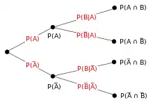
P(A|B) may or may not be equal to P(A) (the unconditional probability of A). If P(A|B) = P(A), then events A and B are said to be independent: in such a case, knowledge about either event does not alter the likelihood of each other. P(A|B) (the conditional probability of A given B) typically differs from P(B|A). For example, if a person has dengue, they might have a 90% chance of testing positive for dengue. In this case, what is being measured is that if event B ("having dengue") has occurred, the probability of A (test is positive) given that B (having dengue) occurred is 90%: that is, P(A|B) = 90%. Alternatively, if a person tests positive for dengue, they may have only a 15% chance of actually having this rare disease, because the false positive rate for the test may be high. In this case, what is being measured is the probability of the event B (having dengue) given that the event A (test is positive) has occurred: P(B|A) = 15%. Falsely equating the two probabilities can lead to various errors of reasoning such as the base rate fallacy. Conditional probabilities can be reversed using Bayes' theorem.
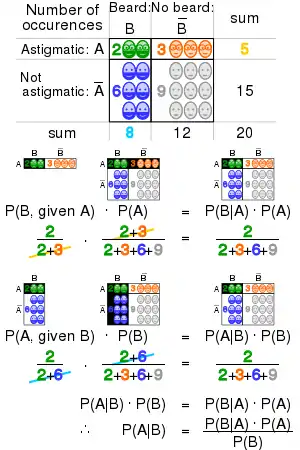
Conditional probabilities can be displayed in a conditional probability table.
Definition


Kolmogorov definition
Given two events A and B from the sigma-field of a probability space, with the unconditional probability of B being greater than zero (i.e., P(B)>0), the conditional probability of A given B is defined to be the quotient of the probability of the joint of events A and B, and the probability of B:[3][6][7]

where is the probability that both events A and B occur. This may be visualized as restricting the sample space to situations in which B occurs. The logic behind this equation is that if the possible outcomes for A and B are restricted to those in which B occurs, this set serves as the new sample space.

Note that the above equation is a definition—not a theoretical result. We just denote the quantity as , and call it the conditional probability of A given B.


As an axiom of probability
Some authors, such as de Finetti, prefer to introduce conditional probability as an axiom of probability:

Although mathematically equivalent, this may be preferred philosophically; under major probability interpretations, such as the subjective theory, conditional probability is considered a primitive entity. Further, this "multiplication axiom" introduces a symmetry with the summation axiom for mutually exclusive events:[8]

As the probability of a conditional event
Conditional probability can be defined as the probability of a conditional event . The Goodman–Nguyen–Van Fraassen conditional event can be defined as


It can be shown that

which meets the Kolmogorov definition of conditional probability.
Conditioning on an event of probability zero
If P(B)=0, then according to the definition, P(A|B) is undefined.
The case of greatest interest is that of a random variable Y, conditioned on a continuous random variable X resulting in a particular outcome x. The event has probability zero and, as such, cannot be conditioned on.

Instead of conditioning on X being exactly x, we could condition on it being closer than distance away from x. The event will generally have nonzero probability and hence, can be conditioned on. We can then take the limit


For example, if two continuous random variables X and Y have a joint density , then by L'Hôpital's rule:


The resulting limit is the conditional probability distribution of Y given X and exists when the denominator, the probability density , is strictly positive.

It is tempting to define the undefined probability using this limit, but this cannot be done in a consistent manner. In particular, it is possible to find random variables X and W and values x, w such that the events and are identical but the resulting limits are not:[9]


The Borel–Kolmogorov paradox demonstrates this with a geometrical argument.
Conditioning on a random variable
Let X be a random variable and its possible outcomes denoted V. For example, if X represents the value of a rolled die then V is the set . Let us assume for the sake of presentation that X is a discrete random variable, so that each value in V has a nonzero probability.

For a value x in V and an event A, the conditional probability is given by . Writing


for short, we see that it is a function of two variables, x and A.
For a fixed A, we can form the random variable . It represents an outcome of whenever a value x of X is observed.

The conditional probability of A given X can thus be treated as a random variable Y with outcomes in the interval . From the law of total probability, its expected value is equal to the unconditional probability of A.

Partial conditional probability
The partial conditional probability is about the probability of event given that each of the condition events has occurred to a degree (degree of belief, degree of experience) that might be different from 100%. Frequentistically, partial conditional probability makes sense, if the conditions are tested in experiment repetitions of appropriate length .[10] Such -bounded partial conditional probability can be defined as the conditionally expected average occurrence of event in testbeds of length that adhere to all of the probability specifications , i.e.:


Based on that, partial conditional probability can be defined as

where [10]

Jeffrey conditionalization[11][12] is a special case of partial conditional probability, in which the condition events must form a partition:

Example
Suppose that somebody secretly rolls two fair six-sided dice, and we wish to compute the probability that the face-up value of the first one is 2, given the information that their sum is no greater than 5.
Probability that D1 = 2
Table 1 shows the sample space of 36 combinations of rolled values of the two dice, each of which occurs with probability 1/36, with the numbers displayed in the red and dark gray cells being D1 + D2.
D1 = 2 in exactly 6 of the 36 outcomes; thus P(D1 = 2) = 6⁄36 = 1⁄6:
Table 1 + D2 1 2 3 4 5 6 D1 1 2 3 4 5 6 7 2 3 4 5 6 7 8 3 4 5 6 7 8 9 4 5 6 7 8 9 10 5 6 7 8 9 10 11 6 7 8 9 10 11 12
Probability that D1 + D2 ≤ 5
Table 2 shows that D1 + D2 ≤ 5 for exactly 10 of the 36 outcomes, thus P(D1 + D2 ≤ 5) = 10⁄36:
Table 2 + D2 1 2 3 4 5 6 D1 1 2 3 4 5 6 7 2 3 4 5 6 7 8 3 4 5 6 7 8 9 4 5 6 7 8 9 10 5 6 7 8 9 10 11 6 7 8 9 10 11 12
Probability that D1 = 2 given that D1 + D2 ≤ 5
Table 3 shows that for 3 of these 10 outcomes, D1 = 2.
Thus, the conditional probability P(D1 = 2 | D1+D2 ≤ 5) = 3⁄10 = 0.3:
Table 3 + D2 1 2 3 4 5 6 D1 1 2 3 4 5 6 7 2 3 4 5 6 7 8 3 4 5 6 7 8 9 4 5 6 7 8 9 10 5 6 7 8 9 10 11 6 7 8 9 10 11 12
Here, in the earlier notation for the definition of conditional probability, the conditioning event B is that D1 + D2 ≤ 5, and the event A is D1 = 2. We have as seen in the table.

Use in inference
In statistical inference, the conditional probability is an update of the probability of an event based on new information.[5] The new information can be incorporated as follows:[1]
- Let A, the event of interest, be in the sample space, say (X,P).
- The occurrence of the event A knowing that event B has or will have occurred, means the occurrence of A as it is restricted to B, i.e. .
- Without the knowledge of the occurrence of B, the information about the occurrence of A would simply be P(A)
- The probability of A knowing that event B has or will have occurred, will be the probability of relative to P(B), the probability that B has occurred.
- This results in whenever P(B) > 0 and 0 otherwise.


This approach results in a probability measure that is consistent with the original probability measure and satisfies all the Kolmogorov axioms. This conditional probability measure also could have resulted by assuming that the relative magnitude of the probability of A with respect to X will be preserved with respect to B (cf. a Formal Derivation below).
The wording "evidence" or "information" is generally used in the Bayesian interpretation of probability. The conditioning event is interpreted as evidence for the conditioned event. That is, P(A) is the probability of A before accounting for evidence E, and P(A|E) is the probability of A after having accounted for evidence E or after having updated P(A). This is consistent with the frequentist interpretation, which is the first definition given above.
Statistical independence
Events A and B are defined to be statistically independent if

If P(B) is not zero, then this is equivalent to the statement that

Similarly, if P(A) is not zero, then

is also equivalent. Although the derived forms may seem more intuitive, they are not the preferred definition as the conditional probabilities may be undefined, and the preferred definition is symmetrical in A and B.
Independent events vs. mutually exclusive events
The concepts of mutually independent events and mutually exclusive events are separate and distinct. The following table contrasts results for the two cases (provided that the probability of the conditioning event is not zero).
| If statistically independent | If mutually exclusive | |
|---|---|---|
| 0 | ||
| 0 | ||
| 0 |


In fact, mutually exclusive events cannot be statistically independent (unless both of them are impossible), since knowing that one occurs gives information about the other (in particular, that the latter will certainly not occur).
Common fallacies
- These fallacies should not be confused with Robert K. Shope's 1978 "conditional fallacy", which deals with counterfactual examples that beg the question.
Assuming conditional probability is of similar size to its inverse
In general, it cannot be assumed that P(A|B) ≈ P(B|A). This can be an insidious error, even for those who are highly conversant with statistics.[13] The relationship between P(A|B) and P(B|A) is given by Bayes' theorem:

That is, P(A|B) ≈ P(B|A) only if P(B)/P(A) ≈ 1, or equivalently, P(A) ≈ P(B).
Assuming marginal and conditional probabilities are of similar size
In general, it cannot be assumed that P(A) ≈ P(A|B). These probabilities are linked through the law of total probability:

where the events form a countable partition of .


This fallacy may arise through selection bias.[14] For example, in the context of a medical claim, let SC be the event that a sequela (chronic disease) S occurs as a consequence of circumstance (acute condition) C. Let H be the event that an individual seeks medical help. Suppose that in most cases, C does not cause S (so that P(SC) is low). Suppose also that medical attention is only sought if S has occurred due to C. From experience of patients, a doctor may therefore erroneously conclude that P(SC) is high. The actual probability observed by the doctor is P(SC|H).
Over- or under-weighting priors
Not taking prior probability into account partially or completely is called base rate neglect. The reverse, insufficient adjustment from the prior probability is conservatism.
Formal derivation
Formally, P(A | B) is defined as the probability of A according to a new probability function on the sample space, such that outcomes not in B have probability 0 and that it is consistent with all original probability measures.[15][16]
Let Ω be a sample space with elementary events {ω}, and let P be the probability measure with respect to the σ-algebra of Ω. Suppose we are told that the event B ⊆ Ω has occurred. A new probability distribution (denoted by the conditional notation) is to be assigned on {ω} to reflect this. All events that are not in B will have null probability in the new distribution. For events in B, two conditions must be met: the probability of B is one and the relative magnitudes of the probabilities must be preserved. The former is required by the axioms of probability, and the latter stems from the fact that the new probability measure has to be the analog of P in which the probability of B is one - and every event that is not in B, therefore, has a null probability. Hence, for some scale factor α, the new distribution must satisfy:

Substituting 1 and 2 into 3 to select α:

So the new probability distribution is

Now for a general event A,

See also
- Bayes' theorem
- Borel–Kolmogorov paradox
- Chain rule (probability)
- Class membership probabilities
- Conditional independence
- Conditional probability distribution
- Conditioning (probability)
- Joint probability distribution
- Monty Hall problem
- Pairwise independent distribution
- Posterior probability
- Regular conditional probability
References
- Gut, Allan (2013). Probability: A Graduate Course (Second ed.). New York, NY: Springer. ISBN 978-1-4614-4707-8.
- "List of Probability and Statistics Symbols". Math Vault. 2020-04-26. Retrieved 2020-09-11.
- "Conditional Probability". www.mathsisfun.com. Retrieved 2020-09-11.
- Ross, Sheldon (2010). A First Course in Probability (8th ed.). Pearson Prentice Hall. ISBN 978-0-13-603313-4.
- Casella, George; Berger, Roger L. (2002). Statistical Inference. Duxbury Press. ISBN 0-534-24312-6.
- Kolmogorov, Andrey (1956), Foundations of the Theory of Probability, Chelsea
- "Conditional Probability". www.stat.yale.edu. Retrieved 2020-09-11.
- Gillies, Donald (2000); "Philosophical Theories of Probability"; Routledge; Chapter 4 "The subjective theory"
- Gal, Yarin. "The Borel–Kolmogorov paradox" (PDF).
- Draheim, Dirk (2017). "Generalized Jeffrey Conditionalization (A Frequentist Semantics of Partial Conditionalization)". Springer. Retrieved December 19, 2017.
- Jeffrey, Richard C. (1983), The Logic of Decision, 2nd edition, University of Chicago Press, ISBN 9780226395821
- "Bayesian Epistemology". Stanford Encyclopedia of Philosophy. 2017. Retrieved December 29, 2017.
- Paulos, J.A. (1988) Innumeracy: Mathematical Illiteracy and its Consequences, Hill and Wang. ISBN 0-8090-7447-8 (p. 63 et seq.)
- Thomas Bruss, F; Der Wyatt Earp Effekt; Spektrum der Wissenschaft; March 2007
- George Casella and Roger L. Berger (1990), Statistical Inference, Duxbury Press, ISBN 0-534-11958-1 (p. 18 et seq.)
- Grinstead and Snell's Introduction to Probability, p. 134
External links
| Wikimedia Commons has media related to Conditional probability. |
- Weisstein, Eric W. "Conditional Probability". MathWorld.
- F. Thomas Bruss Der Wyatt-Earp-Effekt oder die betörende Macht kleiner Wahrscheinlichkeiten (in German), Spektrum der Wissenschaft (German Edition of Scientific American), Vol 2, 110–113, (2007).
- Visual explanation of conditional probability
