Inverse trigonometric functions
In mathematics, the inverse trigonometric functions (occasionally also called arcus functions,[1][2][3][4][5] antitrigonometric functions[6] or cyclometric functions[7][8][9]) are the inverse functions of the trigonometric functions (with suitably restricted domains). Specifically, they are the inverses of the sine, cosine, tangent, cotangent, secant, and cosecant functions,[10][11] and are used to obtain an angle from any of the angle's trigonometric ratios. Inverse trigonometric functions are widely used in engineering, navigation, physics, and geometry.
| Trigonometry |
|---|
 |
| Reference |
| Laws and theorems |
| Calculus |
Notation
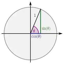
Several notations for the inverse trigonometric functions exist. The most common convention is to name inverse trigonometric functions using an arc- prefix: arcsin(x), arccos(x), arctan(x), etc.[10][6] (This convention is used throughout this article.) This notation arises from the following geometric relationships: when measuring in radians, an angle of θ radians will correspond to an arc whose length is rθ, where r is the radius of the circle. Thus in the unit circle, "the arc whose cosine is x" is the same as "the angle whose cosine is x", because the length of the arc of the circle in radii is the same as the measurement of the angle in radians.[12] In computer programming languages, the inverse trigonometric functions are usually called by the abbreviated forms asin, acos, atan.
The notations sin−1(x), cos−1(x), tan−1(x), etc., as introduced by John Herschel in 1813,[13][14] are often used as well in English-language sources[6]—conventions consistent with the notation of an inverse function. This might appear to conflict logically with the common semantics for expressions such as sin2(x), which refer to numeric power rather than function composition, and therefore may result in confusion between multiplicative inverse or reciprocal and compositional inverse.[15] The confusion is somewhat mitigated by the fact that each of the reciprocal trigonometric functions has its own name—for example, (cos(x))−1 = sec(x). Nevertheless, certain authors advise against using it for its ambiguity.[6][16] Another convention used by a few authors is to use an uppercase first letter, along with a −1 superscript: Sin−1(x), Cos−1(x), Tan−1(x), etc.[17] This potentially avoids confusion with the multiplicative inverse, which should be represented by sin−1(x), cos−1(x), etc.
Since 2009, the ISO 80000-2 standard has specified solely the "arc" prefix for the inverse functions.
Basic properties
Principal values
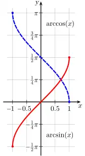
Since none of the six trigonometric functions are one-to-one, they must be restricted in order to have inverse functions. Therefore, the ranges of the inverse functions are proper subsets of the domains of the original functions.
For example, using function in the sense of multivalued functions, just as the square root function y = √x could be defined from y2 = x, the function y = arcsin(x) is defined so that sin(y) = x. For a given real number x, with −1 ≤ x ≤ 1, there are multiple (in fact, countably infinite) numbers y such that sin(y) = x; for example, sin(0) = 0, but also sin(π) = 0, sin(2π) = 0, etc. When only one value is desired, the function may be restricted to its principal branch. With this restriction, for each x in the domain, the expression arcsin(x) will evaluate only to a single value, called its principal value. These properties apply to all the inverse trigonometric functions.
The principal inverses are listed in the following table.
| Name | Usual notation | Definition | Domain of x for real result | Range of usual principal value (radians) |
Range of usual principal value (degrees) |
|---|---|---|---|---|---|
| arcsine | y = arcsin(x) | x = sin(y) | −1 ≤ x ≤ 1 | −π/2 ≤ y ≤ π/2 | −90° ≤ y ≤ 90° |
| arccosine | y = arccos(x) | x = cos(y) | −1 ≤ x ≤ 1 | 0 ≤ y ≤ π | 0° ≤ y ≤ 180° |
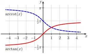
| arctangent | y = arctan(x) | x = tan(y) | all real numbers | −π/2 < y < π/2 | −90° < y < 90° |
| arccotangent | y = arccot(x) | x = cot(y) | all real numbers | 0 < y < π | 0° < y < 180° |
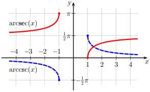
| arcsecant | y = arcsec(x) | x = sec(y) | x ≥ 1 or x ≤ -1 | 0 ≤ y < π/2 or π/2 < y ≤ π | 0° ≤ y < 90° or 90° < y ≤ 180° |
| arccosecant | y = arccsc(x) | x = csc(y) | x ≤ −1 or 1 ≤ x | −π/2 ≤ y < 0 or 0 < y ≤ π/2 | −90° ≤ y < 0° or 0° < y ≤ 90° |
(Note: Some authors define the range of arcsecant to be ( 0 ≤ y < π/2 or π ≤ y < 3π/2 ), because the tangent function is nonnegative on this domain. This makes some computations more consistent. For example, using this range, tan(arcsec(x)) = √x2 − 1, whereas with the range ( 0 ≤ y < π/2 or π/2 < y ≤ π ), we would have to write tan(arcsec(x)) = ±√x2 − 1, since tangent is nonnegative on 0 ≤ y < π/2, but nonpositive on π/2 < y ≤ π. For a similar reason, the same authors define the range of arccosecant to be −π < y ≤ −π/2 or 0 < y ≤ π/2.)
If x is allowed to be a complex number, then the range of y applies only to its real part.
General solutions
Each of the trigonometric functions is periodic in the real part of its argument, running through all its values twice in each interval of 2π:
- Sine and cosecant begin their period at 2πk − π/2 (where k is an integer), finish it at 2πk + π/2, and then reverse themselves over 2πk + π/2 to 2πk + 3π/2.
- Cosine and secant begin their period at 2πk, finish it at 2πk + π, and then reverse themselves over 2πk + π to 2πk + 2π.
- Tangent begins its period at 2πk − π/2, finishes it at 2πk + π/2, and then repeats it (forward) over 2πk + π/2 to 2πk + 3π/2.
- Cotangent begins its period at 2πk, finishes it at 2πk + π, and then repeats it (forward) over 2πk + π to 2πk + 2π.
This periodicity is reflected in the general inverses, where k is some integer.
The following table shows how inverse trigonometric functions may be used to solve equalities involving the six standard trigonometric functions, where it is assumed that r, s, x, and y all lie within the appropriate range.
The symbol ⇔ is logical equality. The expression "LHS ⇔ RHS" indicates that either (a) the left hand side (i.e. LHS) and right hand side (i.e. RHS) are both true, or else (b) the left hand side and right hand side are both false; there is no option (c) (e.g. it is not possible for the LHS statement to be true and also simultaneously for the RHS statement to false), because otherwise "LHS ⇔ RHS" would not have been written (see this footnote[note 1] for an example illustrating this concept).
| Condition | Solution | where... | |
|---|---|---|---|
| sin θ = y | ⇔ | θ = (-1) k arcsin(y) + π k | for some k ∈ ℤ |
| ⇔ | θ = arcsin(y) + 2 π k or θ = - arcsin(y) + 2 π k + π |
for some k ∈ ℤ | |
| csc θ = r | ⇔ | θ = (-1) k arccsc(r) + π k | for some k ∈ ℤ |
| ⇔ | θ = arccsc(y) + 2 π k or θ = - arccsc(y) + 2 π k + π |
for some k ∈ ℤ | |
| cos θ = x | ⇔ | θ = ± arccos(x) + 2 π k | for some k ∈ ℤ |
| ⇔ | θ = arccos(x) + 2 π k or θ = - arccos(x) + 2 π k + π |
for some k ∈ ℤ | |
| sec θ = r | ⇔ | θ = ± arcsec(r) + 2 π k | for some k ∈ ℤ |
| ⇔ | θ = arcsec(x) + 2 π k or θ = - arcsec(x) + 2 π k + 2 π |
for some k ∈ ℤ | |
| tan θ = s | ⇔ | θ = arctan(s) + π k | for some k ∈ ℤ |
| cot θ = r | ⇔ | θ = arccot(r) + π k | for some k ∈ ℤ |
Equal identical trigonometric functions
In the table below, we show how two angles θ and φ must be related, if their values under a given trigonometric function are equal or negatives of each other.
| Equality | Solution | where... | Also a solution to | |||||||||
|---|---|---|---|---|---|---|---|---|---|---|---|---|
| sin θ | = | sin φ | ⇔ | θ = | (-1) k | φ | + | π k | for some k ∈ ℤ | csc θ = csc φ | ||
| cos θ | = | cos φ | ⇔ | θ = | ± | φ | + | 2 | π k | for some k ∈ ℤ | sec θ = sec φ | |
| tan θ | = | tan φ | ⇔ | θ = | φ | + | π k | for some k ∈ ℤ | cot θ = cot φ | |||
| - sin θ | = | sin φ | ⇔ | θ = | (-1) k+1 | φ | + | π k | for some k ∈ ℤ | csc θ = - csc φ | ||
| - cos θ | = | cos φ | ⇔ | θ = | ± | φ | + | 2 | π k | + π | for some k ∈ ℤ | sec θ = - sec φ |
| - tan θ | = | tan φ | ⇔ | θ = | - | φ | + | π k | for some k ∈ ℤ | cot θ = - cot φ | ||
| |sin θ| | = | |sin φ| | ⇔ | θ = | ± | φ | + | π k | for some k ∈ ℤ | |tan θ| = |tan φ| | ||
| ⇕ | |csc θ| = |csc φ| | |||||||||||
| |cos θ| | = | |cos φ| | |sec θ| = |sec φ| | |||||||||
| |cot θ| = |cot φ| | ||||||||||||
Relationships between trigonometric functions and inverse trigonometric functions
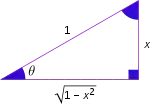
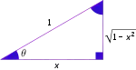
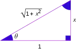
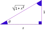
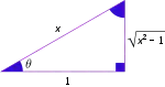
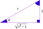
Trigonometric functions of inverse trigonometric functions are tabulated below. A quick way to derive them is by considering the geometry of a right-angled triangle, with one side of length 1 and another side of length x, then applying the Pythagorean theorem and definitions of the trigonometric ratios. Purely algebraic derivations are longer. It's worth noting that for arcsecant and arccosecant, the diagram assumes that x is positive, and thus the result has to be corrected through the use of absolute values and the signum (sgn) operation.
| Diagram | ||||
|---|---|---|---|---|
 | ||||
 | ||||
 | ||||
 | ||||
 | ||||
 | ||||


Relationships among the inverse trigonometric functions
Complementary angles:

Negative arguments:

Reciprocal arguments:

Useful identities if one only has a fragment of a sine table:

Whenever the square root of a complex number is used here, we choose the root with the positive real part (or positive imaginary part if the square was negative real).
A useful form that follows directly from the table above is
- .

It is obtained by recognizing that .

From the half-angle formula, , we get:


Arctangent addition formula

This is derived from the tangent addition formula

by letting

In calculus
Derivatives of inverse trigonometric functions
The derivatives for complex values of z are as follows:

Only for real values of x:

For a sample derivation: if , we get:


Expression as definite integrals
Integrating the derivative and fixing the value at one point gives an expression for the inverse trigonometric function as a definite integral:

When x equals 1, the integrals with limited domains are improper integrals, but still well-defined.
Infinite series
Similar to the sine and cosine functions, the inverse trigonometric functions can also be calculated using power series, as follows. For arcsine, the series can be derived by expanding its derivative, , as a binomial series, and integrating term by term (using the integral definition as above). The series for arctangent can similarly be derived by expanding its derivative in a geometric series, and applying the integral definition above (see Leibniz series).


Series for the other inverse trigonometric functions can be given in terms of these according to the relationships given above. For example, , , and so on. Another series is given by:[18]


Leonhard Euler found a series for the arctangent that converges more quickly than its Taylor series:

(The term in the sum for n = 0 is the empty product, so is 1.)
Alternatively, this can be expressed as

Another series for the arctangent function is given by

where is the imaginary unit.

Continued fractions for arctangent
Two alternatives to the power series for arctangent are these generalized continued fractions:

The second of these is valid in the cut complex plane. There are two cuts, from −i to the point at infinity, going down the imaginary axis, and from i to the point at infinity, going up the same axis. It works best for real numbers running from −1 to 1. The partial denominators are the odd natural numbers, and the partial numerators (after the first) are just (nz)2, with each perfect square appearing once. The first was developed by Leonhard Euler; the second by Carl Friedrich Gauss utilizing the Gaussian hypergeometric series.
Indefinite integrals of inverse trigonometric functions
For real and complex values of z:

For real x ≥ 1:

For all real x not between -1 and 1:

The absolute value is necessary to compensate for both negative and positive values of the arcsecant and arccosecant functions. The signum function is also necessary due to the absolute values in the derivatives of the two functions, which create two different solutions for positive and negative values of x. These can be further simplified using the logarithmic definitions of the inverse hyperbolic functions:

The absolute value in the argument of the arcosh function creates a negative half of its graph, making it identical to the signum logarithmic function shown above.
All of these antiderivatives can be derived using integration by parts and the simple derivative forms shown above.
Example
Using (i.e. integration by parts), set


Then

which by the simple substitution yields the final result:


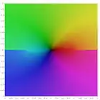
Extension to complex plane
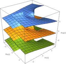
Since the inverse trigonometric functions are analytic functions, they can be extended from the real line to the complex plane. This results in functions with multiple sheets and branch points. One possible way of defining the extension is:

where the part of the imaginary axis which does not lie strictly between the branch points (−i and +i) is the branch cut between the principal sheet and other sheets. The path of the integral must not cross a branch cut. For z not on a branch cut, a straight line path from 0 to z is such a path. For z on a branch cut, the path must approach from Re[x]>0 for the upper branch cut and from Re[x]<0 for the lower branch cut.
The arcsine function may then be defined as:

where (the square-root function has its cut along the negative real axis and) the part of the real axis which does not lie strictly between −1 and +1 is the branch cut between the principal sheet of arcsin and other sheets;

which has the same cut as arcsin;

which has the same cut as arctan;

where the part of the real axis between −1 and +1 inclusive is the cut between the principal sheet of arcsec and other sheets;

which has the same cut as arcsec.
Logarithmic forms
These functions may also be expressed using complex logarithms. This extends their domains to the complex plane in a natural fashion. The following identities for principal values of the functions hold everywhere that they are defined, even on their branch cuts.

Generalization
Because all of the inverse trigonometric functions output an angle of a right triangle, they can be generalized by using Euler's formula to form a right triangle in the complex plane. Algebraically, this gives us:

or

where is the adjacent side, is the opposite side, and is the hypotenuse. From here, we can solve for .


or

Simply taking the imaginary part works for any real-valued and , but if or is complex-valued, we have to use the final equation so that the real part of the result isn't excluded. Since the length of the hypotenuse doesn't change the angle, ignoring the real part of also removes from the equation. In the final equation, we see that the angle of the triangle in the complex plane can be found by inputting the lengths of each side. By setting one of the three sides equal to 1 and one of the remaining sides equal to our input , we obtain a formula for one of the inverse trig functions, for a total of six equations. Because the inverse trig functions require only one input, we must put the final side of the triangle in terms of the other two using the Pythagorean Theorem relation


The table below shows the values of a, b, and c for each of the inverse trig functions and the equivalent expressions for that result from plugging the values into the equations above and simplifying.

In this sense, all of the inverse trig functions can be thought of as specific cases of the complex-valued log function. Since this definition works for any complex-valued , this definition allows for hyperbolic angles as outputs and can be used to further define the inverse hyperbolic functions. Elementary proofs of the relations may also proceed via expansion to exponential forms of the trigonometric functions.
Example proof


Using the exponential definition of sine, one obtains

Let

Solving for


(the positive branch is chosen)

 |
 |
 |
 |
 |
 |


Applications
Application: finding the angle of a right triangle

Inverse trigonometric functions are useful when trying to determine the remaining two angles of a right triangle when the lengths of the sides of the triangle are known. Recalling the right-triangle definitions of sine and cosine, it follows that

Often, the hypotenuse is unknown and would need to be calculated before using arcsine or arccosine using the Pythagorean Theorem: where is the length of the hypotenuse. Arctangent comes in handy in this situation, as the length of the hypotenuse is not needed.


For example, suppose a roof drops 8 feet as it runs out 20 feet. The roof makes an angle θ with the horizontal, where θ may be computed as follows:

Two-argument variant of arctangent
The two-argument atan2 function computes the arctangent of y / x given y and x, but with a range of (−π, π]. In other words, atan2(y, x) is the angle between the positive x-axis of a plane and the point (x, y) on it, with positive sign for counter-clockwise angles (upper half-plane, y > 0), and negative sign for clockwise angles (lower half-plane, y < 0). It was first introduced in many computer programming languages, but it is now also common in other fields of science and engineering.
In terms of the standard arctan function, that is with range of (−π/2, π/2), it can be expressed as follows:

It also equals the principal value of the argument of the complex number x + iy.
This function may also be defined using the tangent half-angle formulae as follows:

provided that either x > 0 or y ≠ 0. However this fails if given x ≤ 0 and y = 0 so the expression is unsuitable for computational use.
The above argument order (y, x) seems to be the most common, and in particular is used in ISO standards such as the C programming language, but a few authors may use the opposite convention (x, y) so some caution is warranted. These variations are detailed at atan2.
Arctangent function with location parameter
In many applications[20] the solution of the equation is to come as close as possible to a given value . The adequate solution is produced by the parameter modified arctangent function


The function rounds to the nearest integer.

Numerical accuracy
For angles near 0 and π, arccosine is ill-conditioned and will thus calculate the angle with reduced accuracy in a computer implementation (due to the limited number of digits).[21] Similarly, arcsine is inaccurate for angles near −π/2 and π/2.
See also
Notes
- To clarify, suppose that it is written "LHS ⇔ RHS" where LHS (which abbreviates "Left Hand Side") and RHS are both statements that can individually be either be true or false. For example, if θ and s are some given and fixed numbers and if the following is written:
- tan θ = s ⇔ θ = arctan(s) + π k for some k ∈ ℤ
References
- Taczanowski, Stefan (1978-10-01). "On the optimization of some geometric parameters in 14 MeV neutron activation analysis". Nuclear Instruments and Methods. ScienceDirect. 155 (3): 543–546. Bibcode:1978NucIM.155..543T. doi:10.1016/0029-554X(78)90541-4.
- Hazewinkel, Michiel (1994) [1987]. Encyclopaedia of Mathematics (unabridged reprint ed.). Kluwer Academic Publishers / Springer Science & Business Media. ISBN 978-155608010-4.
- Ebner, Dieter (2005-07-25). Preparatory Course in Mathematics (PDF) (6 ed.). Department of Physics, University of Konstanz. Archived (PDF) from the original on 2017-07-26. Retrieved 2017-07-26.
- Mejlbro, Leif (2010-11-11). Stability, Riemann Surfaces, Conformal Mappings - Complex Functions Theory (PDF) (1 ed.). Ventus Publishing ApS / Bookboon. ISBN 978-87-7681-702-2. Archived from the original (PDF) on 2017-07-26. Retrieved 2017-07-26.
- Durán, Mario (2012). Mathematical methods for wave propagation in science and engineering. 1: Fundamentals (1 ed.). Ediciones UC. p. 88. ISBN 978-956141314-6.
- Hall, Arthur Graham; Frink, Fred Goodrich (January 1909). "Chapter II. The Acute Angle [14] Inverse trigonometric functions". Written at Ann Arbor, Michigan, USA. Trigonometry. Part I: Plane Trigonometry. New York, USA: Henry Holt and Company / Norwood Press / J. S. Cushing Co. - Berwick & Smith Co., Norwood, Massachusetts, USA. p. 15. Retrieved 2017-08-12.
[…] α = arcsin m: It is frequently read "arc-sine m" or "anti-sine m," since two mutually inverse functions are said each to be the anti-function of the other. […] A similar symbolic relation holds for the other trigonometric functions. […] This notation is universally used in Europe and is fast gaining ground in this country. A less desirable symbol, α = sin-1m, is still found in English and American texts. The notation α = inv sin m is perhaps better still on account of its general applicability. […]
- Klein, Christian Felix (1924) [1902]. Elementarmathematik vom höheren Standpunkt aus: Arithmetik, Algebra, Analysis (in German). 1 (3rd ed.). Berlin: J. Springer.
- Klein, Christian Felix (2004) [1932]. Elementary Mathematics from an Advanced Standpoint: Arithmetic, Algebra, Analysis. Translated by Hedrick, E. R.; Noble, C. A. (Translation of 3rd German ed.). Dover Publications, Inc. / The Macmillan Company. ISBN 978-0-48643480-3. Retrieved 2017-08-13.
- Dörrie, Heinrich (1965). Triumph der Mathematik. Translated by Antin, David. Dover Publications. p. 69. ISBN 978-0-486-61348-2.
- "Comprehensive List of Algebra Symbols". Math Vault. 2020-03-25. Retrieved 2020-08-29.
- Weisstein, Eric W. "Inverse Trigonometric Functions". mathworld.wolfram.com. Retrieved 2020-08-29.
- Beach, Frederick Converse; Rines, George Edwin, eds. (1912). "Inverse trigonometric functions". The Americana: a universal reference library. 21.
- Cajori, Florian (1919). A History of Mathematics (2 ed.). New York, NY: The Macmillan Company. p. 272.
- Herschel, John Frederick William (1813). "On a remarkable Application of Cotes's Theorem". Philosophical Transactions. Royal Society, London. 103 (1): 8. doi:10.1098/rstl.1813.0005.
- "Inverse Trigonometric Functions | Brilliant Math & Science Wiki". brilliant.org. Retrieved 2020-08-29.
- Korn, Grandino Arthur; Korn, Theresa M. (2000) [1961]. "21.2.-4. Inverse Trigonometric Functions". Mathematical handbook for scientists and engineers: Definitions, theorems, and formulars for reference and review (3 ed.). Mineola, New York, USA: Dover Publications, Inc. p. 811. ISBN 978-0-486-41147-7.
- Bhatti, Sanaullah; Nawab-ud-Din; Ahmed, Bashir; Yousuf, S. M.; Taheem, Allah Bukhsh (1999). "Differentiation of Trigonometric, Logarithmic and Exponential Functions". In Ellahi, Mohammad Maqbool; Dar, Karamat Hussain; Hussain, Faheem (eds.). Calculus and Analytic Geometry (1 ed.). Lahore: Punjab Textbook Board. p. 140.
- Borwein, Jonathan; Bailey, David; Gingersohn, Roland (2004). Experimentation in Mathematics: Computational Paths to Discovery (1 ed.). Wellesley, MA, USA: A. K. Peters. p. 51. ISBN 978-1-56881-136-9.
- Hwang Chien-Lih (2005), "An elementary derivation of Euler's series for the arctangent function", The Mathematical Gazette, 89 (516): 469–470, doi:10.1017/S0025557200178404
- when a time varying angle crossing should be mapped by a smooth line instead of a saw toothed one (robotics, astromomy, angular movement in general)
- Gade, Kenneth (2010). "A non-singular horizontal position representation" (PDF). The Journal of Navigation. Cambridge University Press. 63 (3): 395–417. Bibcode:2010JNav...63..395G. doi:10.1017/S0373463309990415.

