Geometric series
In mathematics, a geometric series is the sum of an infinite number of terms that have a constant ratio between successive terms. For example, the series

is geometric, because each successive term can be obtained by multiplying the previous term by 1/2. In general, a geometric series is written as a + ar + ar2 + ar3 + ... , where a is the coefficient of each term and r is the common ratio between adjacent terms. Geometric series are among the simplest examples of infinite series and can serve as a basic introduction to Taylor series and Fourier series. Geometric series had an important role in the early development of calculus, are used throughout mathematics, and have important applications in physics, engineering, biology, economics, computer science, queueing theory, and finance.
The distinction between a progression and a series is that a progression is a sequence, whereas a series is a sum.
Coefficient a
The geometric series a + ar + ar2 + ar3 + ... is written in expanded form.[1] Every coefficient in the geometric series is the same. In contrast, the power series written as a0 + a1r + a2r2 + a3r3 + ... in expanded form has coefficients ai that can vary from term to term. In other words, the geometric series is a special case of the power series. The first term of a geometric series in expanded form is the coefficient a of that geometric series.
In addition to the expanded form of the geometric series, there is a generator form[2] of the geometric series written as
- ark

and a closed form of the geometric series written as
- a / (1 - r) within the range |r| < 1.
The derivation of the closed form from the expanded form is shown in this article's Sum section. The derivation requires that all the coefficients of the series be the same (coefficient a) in order to take advantage of self-similarity and to reduce the infinite number of additions and power operations in the expanded form to the single subtraction and single division in the closed form. However even without that derivation, the result can be confirmed with long division: a divided by (1 - r) results in a + ar + ar2 + ar3 + ... , which is the expanded form of the geometric series.
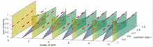
Typically a geometric series is thought of as a sum of numbers a + ar + ar2 + ar3 + ... but can also be thought of as a sum of functions a + ar + ar2 + ar3 + ... that converges to the function a / (1 - r) within the range |r| < 1. The adjacent image shows the contribution each of the first nine terms (i.e., functions) make to the function a / (1 - r) within the range |r| < 1 when a = 1. Changing even one of the coefficients to something other than coefficient a would (in addition to changing the geometric series to a power series) change the resulting sum of functions to some function other than a / (1 - r) within the range |r| < 1. As an aside, a particularly useful change to the coefficients is defined by the Taylor series, which describes how to change the coefficients so that the sum of functions converges to any user selected, sufficiently smooth function within a range.
Common ratio r
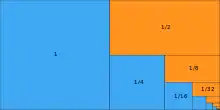
The geometric series a + ar + ar2 + ar3 + ... is an infinite series defined by just two parameters: coefficient a and common ratio r. Common ratio r is the ratio of any term with the previous term in the series. Or equivalently, common ratio r is the term multiplier used to calculate the next term in the series. The following table shows several geometric series:
| a | r | Example series |
|---|---|---|
| 4 | 10 | 4 + 40 + 400 + 4000 + 40,000 + ··· |
| 3 | 1 | 3 + 3 + 3 + 3 + 3 + ··· |
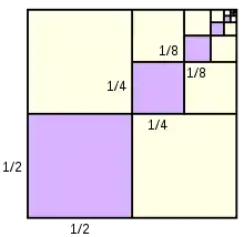
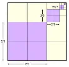
| 1 | 2/3 | 1 + 2/3 + 4/9 + 8/27 + 16/81 + ··· |
| 1/2 | 1/2 | 1/2 + 1/4 + 1/8 + 1/16 + 1/32 + ··· |
| 9 | 1/3 | 9 + 3 + 1 + 1/3 + 1/9 + ··· |
| 7 | 1/10 | 7 + 0.7 + 0.07 + 0.007 + 0.0007 + ··· |
| 1 | −1/2 | 1 − 1/2 + 1/4 − 1/8 + 1/16 − 1/32 + ··· |
| 3 | −1 | 3 − 3 + 3 − 3 + 3 − ··· |
The convergence of the geometric series depends on the value of the common ratio r:
- If |r| < 1, the terms of the series approach zero in the limit (becoming smaller and smaller in magnitude), and the series converges to the sum a / (1 - r).
- If |r| = 1, the series does not converge. When r = 1, all of the terms of the series are the same and the series is infinite. When r = −1, the terms take two values alternately (for example, 2, −2, 2, −2, 2,... ). The sum of the terms oscillates between two values (for example, 2, 0, 2, 0, 2,... ). This is a different type of divergence. See for example Grandi's series: 1 − 1 + 1 − 1 + ···.
- If |r| > 1, the terms of the series become larger and larger in magnitude. The sum of the terms also gets larger and larger, and the series does not converge to a sum. (The series diverges.)
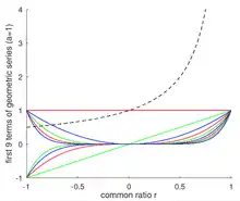
The rate of convergence also depends on the value of the common ratio r. Specifically, the rate of convergence gets slower as r approaches 1 or −1. For example, the geometric series with a = 1 is 1 + r + r2 + r3 + ... and converges to 1 / (1 - r) when |r| < 1. However, the number of terms needed to converge approaches infinity as r approaches 1 because a / (1 - r) approaches infinity and each term of the series is less than or equal to one. In contrast, as r approaches −1 the sum of the first several terms of the geometric series starts to converge to 1/2 but slightly flips up or down depending on whether the most recently added term has a power of r that is even or odd. That flipping behavior near r = −1 is illustrated in the adjacent image showing the first 11 terms of the geometric series with a = 1 and |r| < 1.
The common ratio r and the coefficient a also define the geometric progression, which is a list of the terms of the geometric series but without the additions. Therefore the geometric series a + ar + ar2 + ar3 + ... has the geometric progression (also called the geometric sequence) a, ar, ar2, ar3, ... The geometric progression - as simple as it is - models a surprising number of natural phenomena,
- from some of the largest observations such as the expansion of the universe where the common ratio r is defined by Hubble's constant,
- to some of the smallest observations such as the decay of radioactive carbon-14 atoms where the common ratio r is defined by the half-life of carbon-14.
As an aside, the common ratio r can be a complex number such as |r|eiθ where |r| is the vector's magnitude (or length) and θ is the vector's angle (or orientation) in the complex plane. With a common ratio |r|eiθ, the expanded form of the geometric series is a + a|r|eiθ + a|r|2ei2θ + a|r|3ei3θ + ... Modeling the angle θ as linearly increasing over time at the rate of some angular frequency ω0 (in other words, making the substitution θ = ω0t), the expanded form of the geometric series becomes a + a|r|eiω0t + a|r|2ei2ω0t + a|r|3ei3ω0t + ... , where the first term is a vector of length a not rotating at all, and all the other terms are vectors of different lengths rotating at harmonics of the fundamental angular frequency ω0. The constraint |r|<1 is enough to coordinate this infinite number of vectors of different lengths all rotating at different speeds into tracing a circle, as shown in the adjacent video. Similar to how the Taylor series describes how to change the coefficients so the series converges to a user selected sufficiently smooth function within a range, the Fourier series describes how to change the coefficients (which can also be complex numbers in order to specify the initial angles of vectors) so the series converges to a user selected periodic function.
Sum
Closed-form formula
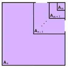
In words, each square is overlapped but can be transformed to a non-overlapped L-shaped area at the next larger square (next power of r) and scaled by 1 / (r - 1) so that the transformation from overlapped square to non-overlapped L-shaped area maintains the same area. Therefore the sum S = Am + Am+1 + ... + An-1 + An = (Lm+1 + Lm+2 + ... + Ln + Ln+1) / (r - 1). Observe that the non-overlapped L-shaped areas from L-shaped area m + 1 to L-shaped area n + 1 are a partition of the non-overlapped square An+1 less the upper right square notch Am (because there are no overlapped smaller squares to be transformed into that notch of area Am). Therefore, substituting Ai = ri and scaling all the terms by coefficient a results in the general, closed-form, geometric series S = (rn+1 - rm) a / (r - 1) when m < n and r > 1.
Although the above geometric proof assumes r > 1, the same closed form formula can be shown to apply to any value of r with the possible exception of r = 0 (depending on how you choose to define zero to the power of zero). For example for the case of r = 1, S = (1n+1 - 1m) a / (1 - 1) = 0 / 0. However, applying L'Hôpital's rule results in S = (n + 1 - m) a when r = 1. For the case of 0 < r < 1, start with S = (rn+1 - rm) a / (r - 1) when m < n, r > 1 and let m = -∞ and n = 0 so S = ar / (r - 1) when r > 1. Dividing the numerator and denominator by r gives S = a / (1 - (1/r)) when r > 1, which is equivalent to S = a / (1 - r) when 0 < r < 1 because inverting r reverses the order of the series (biggest to smallest instead of smallest to biggest) but does not change the sum. The range 0 < r < 1 can be extended to the range -1 < r < 1 by applying the derived formula, S = a / (1 - r) when 0 < r < 1, separately to two partitions of the geometric series: one with even powers of r (which cannot be negative) and the other with odd powers of r (which can be negative). The sum over both partitions is S = a / (1 - r2) + ar / (1 - r2) = a (1 + r) / ((1 + r)(1 - r)) = a / (1 - r).
For , the sum of the first n+1 terms of a geometric series, up to and including the r n term, is


where r is the common ratio. One can derive that closed-form formula for the partial sum, s, by subtracting out the many self-similar terms as follows:[3][4][5]

As n approaches infinity, the absolute value of r must be less than one for the series to converge. The sum then becomes

When a = 1, this can be simplified to

The formula also holds for complex r, with the corresponding restriction, the modulus of r is strictly less than one.
As an aside, the question of whether an infinite series converges is fundamentally a question about the distance between two values: given enough terms, does the value of the partial sum get arbitrarily close to the value it is approaching? In the above derivation of the closed form of the geometric series, the interpretation of the distance between two values is the distance between their locations on the number line. That is the most common interpretation of distance between two values. However the p-adic metric, which has become a critical notion in modern number theory, offers a definition of distance such that the geometric series 1 + 2 + 4 + 8 + ... with a = 1 and r = 2 actually does converge to a / (1 - r) = 1 / (1 - 2) = -1 even though r is outside the typical convergence range |r| < 1.
Proof of convergence
We can prove that the geometric series converges using the sum formula for a geometric progression:

Since (1 + r + r2 + ... + rn)(1−r)
= ((1-r) + (r - r2) + (r2 - r3) + ... + (rn - rn+1))
= ((1-r) + (r - r2) + (r2 - r3) + ... + (rn - rn+1))
= 1−rn+1 and rn+1 → 0 for | r | < 1.
Convergence of geometric series can also be demonstrated by rewriting the series as an equivalent telescoping series. Consider the function,

Note that

Thus,

If

then

So S converges to

Rate of convergence
As shown in the above proofs, the closed form of the geometric series partial sum up to and including the n-th power of r is a(1 - rn+1) / (1 - r) for any value of r, and the closed form of the geometric series is the full sum a / (1 - r) within the range |r| < 1.
If the common ratio is within the range 0 < r < 1, then the partial sum a(1 - rn+1) / (1 - r) increases with each added term and eventually gets within some small error, E, ratio of the full sum a / (1 - r). Solving for n at that error threshold,

where 0 < r < 1, the ceiling operation constrains n to integers, and the natural log operation ln flips the inequality because it negates both sides of the inequality (because both sides are less than one). The result n+1 is the number of partial sum terms needed to get within aE / (1 - r) of the full sum a / (1 - r). For example to get within 1% of the full sum a / (1 - r) at r=0.1, only 2 (= ln(E) / ln(r) = ln(0.01) / ln(0.1)) terms of the partial sum are needed. However at r=0.9, 44 (= ln(0.01) / ln(0.9)) terms of the partial sum are needed to get within 1% of the full sum a / (1 - r).

If the common ratio is within the range -1 < r < 0, then the geometric series is an alternating series but can be converted into the form of a non-alternating geometric series by combining pairs of terms and then analyzing the rate of convergence using the same approach as shown for the common ratio range 0 < r < 1. Specifically, the partial sum
- s = a + ar + ar2 + ar3 + ar4 + ar5 + ... + arn-1 + arn within the range -1 < r < 0 is equivalent to
- s = a - ap + ap2 - ap3 + ap4 - ap5 + ... + apn-1 - apn with an n that is odd, with the substitution of p = -r, and within the range 0 < p < 1,
- s = (a - ap) + (ap2 - ap3) + (ap4 - ap5) + ... + (apn-1 - apn) with adjacent and differently signed terms paired together,
- s = a(1 - p) + a(1 - p)p2 + a(1 - p)p4 + ... + a(1 - p)p2(n-1)/2 with a(1 - p) factored out of each term,
- s = a(1 - p) + a(1 - p)p2 + a(1 - p)p4 + ... + a(1 - p)p2m with the substitution m = (n - 1) / 2 which is an integer given the constraint that n is odd,
which is now in the form of the first m terms of a geometric series with coefficient a(1 - p) and with common ratio p2. Therefore the closed form of the partial sum is a(1 - p)(1 - p2(m+1)) / (1 - p2) which increases with each added term and eventually gets within some small error, E, ratio of the full sum a(1 - p) / (1 - p2). As before, solving for m at that error threshold,

where 0 < p < 1 or equivalently -1 < r < 0, and the m+1 result is the number of partial sum pairs of terms needed to get within a(1 - p)E / (1 - p2) of the full sum a(1 - p) / (1 - p2). For example to get within 1% of the full sum a(1 - p) / (1 - p2) at p=0.1 or equivalently r=-0.1, only 1 (= ln(E) / (2 ln(p)) = ln(0.01) / (2 ln(0.1)) pair of terms of the partial sum are needed. However at p=0.9 or equivalently r=-0.9, 22 (= ln(0.01) / (2 ln(0.9))) pairs of terms of the partial sum are needed to get within 1% of the full sum a(1 - p) / (1 - p2). Comparing the rate of convergence for positive and negative values of r, n + 1 (the number of terms required to reach the error threshold for some positive r) is always twice as large as m + 1 (the number of term pairs required to reach the error threshold for the negative of that r) but the m + 1 refers to term pairs instead of single terms. Therefore, the rate of convergence is symmetric about r = 0, which can be a surprise given the asymmetry of a / (1 - r). One perspective that helps explain this rate of convergence symmetry is that on the r > 0 side each added term of the partial sum makes a finite contribution to the infinite sum at r = 1 while on the r < 0 side each added term makes a finite contribution to the infinite slope at r = -1.
As an aside, this type of rate of convergence analysis is particularly useful when calculating the number of Taylor series terms needed to adequately approximate some user-selected sufficiently-smooth function or when calculating the number of Fourier series terms needed to adequately approximate some user-selected periodic function.
Historic insights
Euclid
Book IX, Proposition 35[6] of Euclid's Elements expresses the partial sum of a geometric series in terms of members of the series. It is equivalent to the modern formula.
Archimedes' quadrature of the parabola
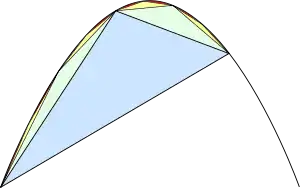
Archimedes used the sum of a geometric series to compute the area enclosed by a parabola and a straight line. His method was to dissect the area into an infinite number of triangles.
Archimedes' Theorem states that the total area under the parabola is 4/3 of the area of the blue triangle.
Archimedes determined that each green triangle has 1/8 the area of the blue triangle, each yellow triangle has 1/8 the area of a green triangle, and so forth.
Assuming that the blue triangle has area 1, the total area is an infinite sum:

The first term represents the area of the blue triangle, the second term the areas of the two green triangles, the third term the areas of the four yellow triangles, and so on. Simplifying the fractions gives

This is a geometric series with common ratio 1/4 and the fractional part is equal to

The sum is

This computation uses the method of exhaustion, an early version of integration. Using calculus, the same area could be found by a definite integral.
Applications
Repeating decimals
A repeating decimal can be thought of as a geometric series whose common ratio is a power of 1/10. For example:

The formula for the sum of a geometric series can be used to convert the decimal to a fraction,

The formula works not only for a single repeating figure, but also for a repeating group of figures. For example:

Note that every series of repeating consecutive decimals can be conveniently simplified with the following:


That is, a repeating decimal with repeat length n is equal to the quotient of the repeating part (as an integer) and 10n - 1.
Economics
In economics, geometric series are used to represent the present value of an annuity (a sum of money to be paid in regular intervals).
For example, suppose that a payment of $100 will be made to the owner of the annuity once per year (at the end of the year) in perpetuity. Receiving $100 a year from now is worth less than an immediate $100, because one cannot invest the money until one receives it. In particular, the present value of $100 one year in the future is $100 / (1 + ), where is the yearly interest rate.

Similarly, a payment of $100 two years in the future has a present value of $100 / (1 + )2 (squared because two years' worth of interest is lost by not receiving the money right now). Therefore, the present value of receiving $100 per year in perpetuity is

which is the infinite series:

This is a geometric series with common ratio 1 / (1 + ). The sum is the first term divided by (one minus the common ratio):

For example, if the yearly interest rate is 10% ( = 0.10), then the entire annuity has a present value of $100 / 0.10 = $1000.
This sort of calculation is used to compute the APR of a loan (such as a mortgage loan). It can also be used to estimate the present value of expected stock dividends, or the terminal value of a security.
Fractal geometry
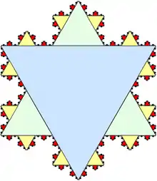
In the study of fractals, geometric series often arise as the perimeter, area, or volume of a self-similar figure.
For example, the area inside the Koch snowflake can be described as the union of infinitely many equilateral triangles (see figure). Each side of the green triangle is exactly 1/3 the size of a side of the large blue triangle, and therefore has exactly 1/9 the area. Similarly, each yellow triangle has 1/9 the area of a green triangle, and so forth. Taking the blue triangle as a unit of area, the total area of the snowflake is

The first term of this series represents the area of the blue triangle, the second term the total area of the three green triangles, the third term the total area of the twelve yellow triangles, and so forth. Excluding the initial 1, this series is geometric with constant ratio r = 4/9. The first term of the geometric series is a = 3(1/9) = 1/3, so the sum is

Thus the Koch snowflake has 8/5 of the area of the base triangle.
Zeno's paradoxes
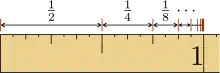
The convergence of a geometric series reveals that a sum involving an infinite number of summands can indeed be finite, and so allows one to resolve many of Zeno's paradoxes. For example, Zeno's dichotomy paradox maintains that movement is impossible, as one can divide any finite path into an infinite number of steps wherein each step is taken to be half the remaining distance. Zeno's mistake is in the assumption that the sum of an infinite number of finite steps cannot be finite. This is of course not true, as evidenced by the convergence of the geometric series with .

This, however, is not a complete resolution to Zeno's dichotomy paradox. Strictly speaking, unless we allow for time to move in reverse, where the step size begins with and approaches zero as a limit, this infinite series would otherwise have to begin with an infinitesimally small step. Treating infinitesimals in this way is typically not something which is rigorously defined mathematically, outside of Nonstandard Calculus. So, while it is true that the entire infinite summation yields a finite number, we can not create a simple ordering of the terms when starting from an infinitesimal, and therefore we can not adequately describe the first step of any given action.
Geometric power series
The formula for a geometric series

can be interpreted as a power series in the Taylor's theorem sense, converging where . From this, one can extrapolate to obtain other power series. For example,


By differentiating the geometric series, one obtains the variant[7]

Similarly obtained are:
- and


See also
| Part of a series of articles about |
| Calculus |
|---|
- 0.999... – Alternative decimal expansion of the number 1
- Asymptote – In geometry, limit of the tangent at a point that tends to infinity
- Divergent geometric series
- Generalized hypergeometric function
- Geometric progression
- Neumann series
- Ratio test
- Root test
- Series (mathematics) – Infinite sum
Specific geometric series
- Grandi's series: 1 − 1 + 1 − 1 + ⋯
- 1 + 2 + 4 + 8 + ⋯
- 1 − 2 + 4 − 8 + ⋯
- 1/2 + 1/4 + 1/8 + 1/16 + ⋯
- 1/2 − 1/4 + 1/8 − 1/16 + ⋯
- 1/4 + 1/16 + 1/64 + 1/256 + ⋯
- A geometric series is a unit series (the series sum converges to one) if and only if |r| < 1 and a + r = 1 (equivalent to the more familiar form S = a / (1 - r) = 1 when |r| < 1). Therefore, an alternating series is also a unit series when -1 < r < 0 and a + r = 1 (for example, coefficient a = 1.7 and common ratio r = -0.7).
- The terms of a geometric series are also the terms of a generalized Fibonacci sequence (Fn = Fn-1 + Fn-2 but without requiring F0 = 0 and F1 = 1) when a geometric series common ratio r satisfies the constraint 1 + r = r2, which according to the quadratic formula is when the common ratio r equals the golden ratio (i.e., common ratio r = (1 ± √5)/2).
- The only geometric series that is a unit series and also has terms of a generalized Fibonacci sequence has the golden ratio as its coefficient a and the conjugate golden ratio as its common ratio r (i.e., a = (1 + √5)/2 and r = (1 - √5)/2). It is a unit series because a + r = 1 and |r| < 1, it is a generalized Fibonacci sequence because 1 + r = r2, and it is an alternating series because r < 0.
Notes
- Riddle, Douglas F. Calculus and Analytic Geometry, Second Edition Belmont, California, Wadsworth Publishing, p. 566, 1970.
- Riddle, Douglas F. Calculus and Analytic Geometry, Second Edition Belmont, California, Wadsworth Publishing, p. 566, 1970.
- Abramowitz & Stegun (1972, p. 10)
- Moise (1967, p. 48)
- Protter & Morrey (1970, pp. 639–640)
- "Euclid's Elements, Book IX, Proposition 35". Aleph0.clarku.edu. Retrieved 2013-08-01.
- Taylor, Angus E. (1955). Advanced Calculus. Blaisdell. p. 603.
References
- Abramowitz, M. and Stegun, I. A. (Eds.). Handbook of Mathematical Functions with Formulas, Graphs, and Mathematical Tables, 9th printing. New York: Dover, p. 10, 1972.
- Andrews, George E. (1998). "The geometric series in calculus". The American Mathematical Monthly. Mathematical Association of America. 105 (1): 36–40. doi:10.2307/2589524. JSTOR 2589524.
- Arfken, G. Mathematical Methods for Physicists, 3rd ed. Orlando, FL: Academic Press, pp. 278–279, 1985.
- Beyer, W. H. CRC Standard Mathematical Tables, 28th ed. Boca Raton, FL: CRC Press, p. 8, 1987.
- Courant, R. and Robbins, H. "The Geometric Progression." §1.2.3 in What Is Mathematics?: An Elementary Approach to Ideas and Methods, 2nd ed. Oxford, England: Oxford University Press, pp. 13–14, 1996.
- James Stewart (2002). Calculus, 5th ed., Brooks Cole. ISBN 978-0-534-39339-7
- Larson, Hostetler, and Edwards (2005). Calculus with Analytic Geometry, 8th ed., Houghton Mifflin Company. ISBN 978-0-618-50298-1
- Moise, Edwin E. (1967), Calculus: Complete, Reading: Addison-Wesley
- Pappas, T. "Perimeter, Area & the Infinite Series." The Joy of Mathematics. San Carlos, CA: Wide World Publ./Tetra, pp. 134–135, 1989.
- Protter, Murray H.; Morrey, Charles B., Jr. (1970), College Calculus with Analytic Geometry (2nd ed.), Reading: Addison-Wesley, LCCN 76087042
- Roger B. Nelsen (1997). Proofs without Words: Exercises in Visual Thinking, The Mathematical Association of America. ISBN 978-0-88385-700-7
History and philosophy
- C. H. Edwards, Jr. (1994). The Historical Development of the Calculus, 3rd ed., Springer. ISBN 978-0-387-94313-8.
- Swain, Gordon and Thomas Dence (April 1998). "Archimedes' Quadrature of the Parabola Revisited". Mathematics Magazine. 71 (2): 123–30. doi:10.2307/2691014. JSTOR 2691014.
- Eli Maor (1991). To Infinity and Beyond: A Cultural History of the Infinite, Princeton University Press. ISBN 978-0-691-02511-7
- Morr Lazerowitz (2000). The Structure of Metaphysics (International Library of Philosophy), Routledge. ISBN 978-0-415-22526-7
Economics
Biology
Computer science
- John Rast Hubbard (2000). Schaum's Outline of Theory and Problems of Data Structures With Java, McGraw-Hill. ISBN 978-0-07-137870-3
External links
- "Geometric progression", Encyclopedia of Mathematics, EMS Press, 2001 [1994]
- Weisstein, Eric W. "Geometric Series". MathWorld.
- Geometric Series at PlanetMath.
- Peppard, Kim. "College Algebra Tutorial on Geometric Sequences and Series". West Texas A&M University.
- Casselman, Bill. "A Geometric Interpretation of the Geometric Series". Archived from the original (Applet) on 2007-09-29.
- "Geometric Series" by Michael Schreiber, Wolfram Demonstrations Project, 2007.