Proper orthogonal decomposition
The Proper Orthogonal Decomposition is a numerical method commonly applied to the field of Finite Element Simulation.
| Part of a series on |
| Machine learning and data mining |
|---|
It enables to reduce the complexity of compute intensive simulation such as Computational Fluid Dynamics and Structural Analysis (like Crash Simulation). Typically in Fluid Dynamics and turbulences analysis, it is used to replace the Navier-Stokes equations by simpler models to solve.[1]
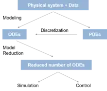
It belongs to a class of algorithms called Model Order Reduction (or in short Model Reduction). What it essentially does is to train a model based on simulation data. To this extent, it can be associated with the field of machine learning.
POD and PCA
The main use of POD is to decompose a physical field (like Pressure, Temperature in Fluid Dynamics or Stress and Deformation in Structural Analysis), depending on the different variables that influence its physical behaviors. As its name hints, it's operating an Orthogonal Decomposition along with the Principal Components of the field. As such it is assimilated with the Principal Component Analysis from Pearson in the field of statistics, or the Singular Value Decomposition in linear algebra because it refers to eigenvalues and eigenvectors of a physical field. In those domains, it is associated with the research of Karhunen[2] and Loève,[3] and their Karhunen–Loève theorem.
Mathematical expression
The first idea behind the Proper Orthogonal Decomposition (POD), as it was originally formulated in the domain of fluid dynamics to analyze turbulences, is to decompose a random vector field u(x, t) into a set of deterministic spatial functions Φk(x) modulated by random time coefficients ak(t) so that:

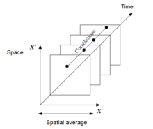
The first step is to sample the vector field over a period of time in what we call snapshots (as display in the image of the POD snapshots). This snapshot method[4] is averaging the samples over the space dimension n, and correlating them with each other along the time samples p:
with n spatial elements, and p time samples

The next step is to compute the covariance matrix C

We then compute the eigenvalues and eigenvectors of C and we order them from the largest eigenvalue to the smallest.
We obtain n eigenvalues λ1...λn and a set of n eigenvectors arranged as columns in an n × n matrix Φ:

Courses on POD
- MIT: http://web.mit.edu/6.242/www/images/lec6_6242_2004.pdf
- Stanford University - Charbel Farhat & David Amsallem https://web.stanford.edu/group/frg/course_work/CME345/CA-CME345-Ch4.pdf
- Weiss, Julien: A Tutorial on the Proper Orthogonal Decomposition. In: 2019 AIAA Aviation Forum. 17–21 June 2019, Dallas, Texas, United States.
- French course from CNRS https://www.math.u-bordeaux.fr/~mbergman/PDF/OuvrageSynthese/OCET06.pdf
- Applications of the Proper Orthogonal Decomposition Method http://www.cerfacs.fr/~cfdbib/repository/WN_CFD_07_97.pdf
References
- Berkooz, G; Holmes, P; Lumley, J L (January 1993). "The Proper Orthogonal Decomposition in the Analysis of Turbulent Flows". Annual Review of Fluid Mechanics. 25 (1): 539–575. doi:10.1146/annurev.fl.25.010193.002543. ISSN 0066-4189.
- Karhunen, Kari (1946). Zur spektral theorie stochasticher prozesse.
- David, F. N.; Loeve, M. (December 1955). "Probability Theory". Biometrika. 42 (3/4): 540. doi:10.2307/2333409. ISSN 0006-3444.
- Sirovich, Lawrence (1987-10-01). "Turbulence and the dynamics of coherent structures. I. Coherent structures". Quarterly of Applied Mathematics. 45 (3): 561–571. doi:10.1090/qam/910462. ISSN 0033-569X.
