Time complexity
In computer science, the time complexity is the computational complexity that describes the amount of computer time it takes to run an algorithm. Time complexity is commonly estimated by counting the number of elementary operations performed by the algorithm, supposing that each elementary operation takes a fixed amount of time to perform. Thus, the amount of time taken and the number of elementary operations performed by the algorithm are taken to differ by at most a constant factor.
Since an algorithm's running time may vary among different inputs of the same size, one commonly considers the worst-case time complexity, which is the maximum amount of time required for inputs of a given size. Less common, and usually specified explicitly, is the average-case complexity, which is the average of the time taken on inputs of a given size (this makes sense because there are only a finite number of possible inputs of a given size). In both cases, the time complexity is generally expressed as a function of the size of the input.[1]:226 Since this function is generally difficult to compute exactly, and the running time for small inputs is usually not consequential, one commonly focuses on the behavior of the complexity when the input size increases—that is, the asymptotic behavior of the complexity. Therefore, the time complexity is commonly expressed using big O notation, typically etc., where n is the input size in units of bits needed to represent the input.


Algorithmic complexities are classified according to the type of function appearing in the big O notation. For example, an algorithm with time complexity is a linear time algorithm and an algorithm with time complexity for some constant is a polynomial time algorithm.


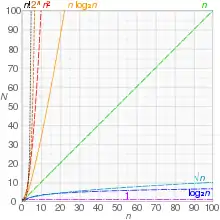
Table of common time complexities
The following table summarizes some classes of commonly encountered time complexities. In the table, poly(x) = xO(1), i.e., polynomial in x.
| Name | Complexity class | Running time (T(n)) | Examples of running times | Example algorithms |
|---|---|---|---|---|
| constant time | O(1) | 10 | Finding the median value in a sorted array of numbers
Calculating (−1)n | |
| inverse Ackermann time | O(α(n)) | Amortized time per operation using a disjoint set | ||
| iterated logarithmic time | O(log* n) | Distributed coloring of cycles | ||
| log-logarithmic | O(log log n) | Amortized time per operation using a bounded priority queue[2] | ||
| logarithmic time | DLOGTIME | O(log n) | log n, log(n2) | Binary search |
| polylogarithmic time | poly(log n) | (log n)2 | ||
| fractional power | O(nc) where 0 < c < 1 | n1/2, n2/3 | Searching in a kd-tree | |
| linear time | O(n) | n, 2n + 5 | Finding the smallest or largest item in an unsorted array, Kadane's algorithm, linear search | |
| "n log-star n" time | O(n log* n) | Seidel's polygon triangulation algorithm. | ||
| linearithmic time | O(n log n) | n log n, log n! | Fastest possible comparison sort; Fast Fourier transform. | |
| quasilinear time | n poly(log n) | |||
| quadratic time | O(n2) | n2 | Bubble sort; Insertion sort; Direct convolution | |
| cubic time | O(n3) | n3 | Naive multiplication of two n×n matrices. Calculating partial correlation. | |
| polynomial time | P | 2O(log n) = poly(n) | n2 + n, n10 | Karmarkar's algorithm for linear programming; AKS primality test[3][4] |
| quasi-polynomial time | QP | 2poly(log n) | nlog log n, nlog n | Best-known O(log2 n)-approximation algorithm for the directed Steiner tree problem. |
| sub-exponential time (first definition) | SUBEXP | O(2nε) for all ε > 0 | Contains BPP unless EXPTIME (see below) equals MA.[5] | |
| sub-exponential time (second definition) | 2o(n) | 2n1/3 | Best-known algorithm for integer factorization; formerly-best algorithm for graph isomorphism | |
| exponential time (with linear exponent) | E | 2O(n) | 1.1n, 10n | Solving the traveling salesman problem using dynamic programming |
| exponential time | EXPTIME | 2poly(n) | 2n, 2n2 | Solving matrix chain multiplication via brute-force search |
| factorial time | O(n!) | n! | Solving the traveling salesman problem via brute-force search | |
| double exponential time | 2-EXPTIME | 22poly(n) | 22n | Deciding the truth of a given statement in Presburger arithmetic |
Constant time
An algorithm is said to be constant time (also written as O(1) time) if the value of T(n) is bounded by a value that does not depend on the size of the input. For example, accessing any single element in an array takes constant time as only one operation has to be performed to locate it. In a similar manner, finding the minimal value in an array sorted in ascending order; it is the first element. However, finding the minimal value in an unordered array is not a constant time operation as scanning over each element in the array is needed in order to determine the minimal value. Hence it is a linear time operation, taking O(n) time. If the number of elements is known in advance and does not change, however, such an algorithm can still be said to run in constant time.
Despite the name "constant time", the running time does not have to be independent of the problem size, but an upper bound for the running time has to be bounded independently of the problem size. For example, the task "exchange the values of a and b if necessary so that a≤b" is called constant time even though the time may depend on whether or not it is already true that a ≤ b. However, there is some constant t such that the time required is always at most t.
Here are some examples of code fragments that run in constant time :
int index = 5;
int item = list[index];
if (condition true) then
    perform some operation that runs in constant time
else
    perform some other operation that runs in constant time
for i = 1 to 100
    for j = 1 to 200
        perform some operation that runs in constant time
If T(n) is O(any constant value), this is equivalent to and stated in standard notation as T(n) being O(1).
Logarithmic time
An algorithm is said to take logarithmic time when T(n) = O(log n). Since loga n and logb n are related by a constant multiplier, and such a multiplier is irrelevant to big-O classification, the standard usage for logarithmic-time algorithms is O(log n) regardless of the base of the logarithm appearing in the expression of T.
Algorithms taking logarithmic time are commonly found in operations on binary trees or when using binary search.
An O(log n) algorithm is considered highly efficient, as the ratio of the number of operations to the size of the input decreases and tends to zero when n increases. An algorithm that must access all elements of its input cannot take logarithmic time, as the time taken for reading an input of size n is of the order of n.
An example of logarithmic time is given by dictionary search. Consider a dictionary D which contains n entries, sorted by alphabetical order. We suppose that, for 1 ≤ k ≤ n, one may access the kth entry of the dictionary in a constant time. Let D(k) denote this k-th entry. Under these hypotheses, the test to see if a word w is in the dictionary may be done in logarithmic time: consider where denotes the floor function. If then we are done. Else, if continue the search in the same way in the left half of the dictionary, otherwise continue similarly with the right half of the dictionary. This algorithm is similar to the method often used to find an entry in a paper dictionary.


Polylogarithmic time
An algorithm is said to run in polylogarithmic time if its time T(n) is O((log n)k) for some constant k. Another way to write this is O(logk n).
For example, matrix chain ordering can be solved in polylogarithmic time on a parallel random-access machine,[6] and a graph can be determined to be planar in a fully dynamic way in O(log3 n) time per insert/delete operation.[7]
Sub-linear time
An algorithm is said to run in sub-linear time (often spelled sublinear time) if T(n) = o(n). In particular this includes algorithms with the time complexities defined above.
Typical algorithms that are exact and yet run in sub-linear time use parallel processing (as the NC1 matrix determinant calculation does), or alternatively have guaranteed assumptions on the input structure (as the logarithmic time binary search and many tree maintenance algorithms do). However, formal languages such as the set of all strings that have a 1-bit in the position indicated by the first log(n) bits of the string may depend on every bit of the input and yet be computable in sub-linear time.
The specific term sublinear time algorithm is usually reserved to algorithms that are unlike the above in that they are run over classical serial machine models and are not allowed prior assumptions on the input.[8] They are however allowed to be randomized, and indeed must be randomized for all but the most trivial of tasks.
As such an algorithm must provide an answer without reading the entire input, its particulars heavily depend on the access allowed to the input. Usually for an input that is represented as a binary string b1,...,bk it is assumed that the algorithm can in time O(1) request and obtain the value of bi for any i.
Sub-linear time algorithms are typically randomized, and provide only approximate solutions. In fact, the property of a binary string having only zeros (and no ones) can be easily proved not to be decidable by a (non-approximate) sub-linear time algorithm. Sub-linear time algorithms arise naturally in the investigation of property testing.
Linear time
An algorithm is said to take linear time, or O(n) time, if its time complexity is O(n). Informally, this means that the running time increases at most linearly with the size of the input. More precisely, this means that there is a constant c such that the running time is at most cn for every input of size n. For example, a procedure that adds up all elements of a list requires time proportional to the length of the list, if the adding time is constant, or, at least, bounded by a constant.
Linear time is the best possible time complexity in situations where the algorithm has to sequentially read its entire input. Therefore, much research has been invested into discovering algorithms exhibiting linear time or, at least, nearly linear time. This research includes both software and hardware methods. There are several hardware technologies which exploit parallelism to provide this. An example is content-addressable memory. This concept of linear time is used in string matching algorithms such as the Boyer–Moore algorithm and Ukkonen's algorithm.
Quasilinear time
An algorithm is said to run in quasilinear time (also referred to as log-linear time) if T(n) = O(n logk n) for some positive constant k;[9] linearithmic time is the case k = 1.[10] Using soft O notation these algorithms are Õ(n). Quasilinear time algorithms are also O(n1+ε) for every constant ε > 0, and thus run faster than any polynomial time algorithm whose time bound includes a term nc for any c > 1.
Algorithms which run in quasilinear time include:
- In-place merge sort, O(n log2 n)
- Quicksort, O(n log n), in its randomized version, has a running time that is O(n log n) in expectation on the worst-case input. Its non-randomized version has an O(n log n) running time only when considering average case complexity.
- Heapsort, O(n log n), merge sort, introsort, binary tree sort, smoothsort, patience sorting, etc. in the worst case
- Fast Fourier transforms, O(n log n)
- Monge array calculation, O(n log n)
In many cases, the n · log n running time is simply the result of performing a Θ(log n) operation n times (for the notation, see Big O notation § Family of Bachmann–Landau notations). For example, binary tree sort creates a binary tree by inserting each element of the n-sized array one by one. Since the insert operation on a self-balancing binary search tree takes O(log n) time, the entire algorithm takes O(n log n) time.
Comparison sorts require at least Ω(n log n) comparisons in the worst case because log(n!) = Θ(n log n), by Stirling's approximation. They also frequently arise from the recurrence relation T(n) = 2T(n/2) + O(n).
Sub-quadratic time
An algorithm is said to be subquadratic time if T(n) = o(n2).
For example, simple, comparison-based sorting algorithms are quadratic (e.g. insertion sort), but more advanced algorithms can be found that are subquadratic (e.g. shell sort). No general-purpose sorts run in linear time, but the change from quadratic to sub-quadratic is of great practical importance.
Polynomial time
An algorithm is said to be of polynomial time if its running time is upper bounded by a polynomial expression in the size of the input for the algorithm, i.e., T(n) = O(nk) for some positive constant k.[1][11] Problems for which a deterministic polynomial time algorithm exists belong to the complexity class P, which is central in the field of computational complexity theory. Cobham's thesis states that polynomial time is a synonym for "tractable", "feasible", "efficient", or "fast".[12]
Some examples of polynomial time algorithms:
- The selection sort sorting algorithm on n integers performs operations for some constant A. Thus it runs in time and is a polynomial time algorithm.
- All the basic arithmetic operations (addition, subtraction, multiplication, division, and comparison) can be done in polynomial time.
- Maximum matchings in graphs can be found in polynomial time.


Strongly and weakly polynomial time
In some contexts, especially in optimization, one differentiates between strongly polynomial time and weakly polynomial time algorithms. These two concepts are only relevant if the inputs to the algorithms consist of integers.
Strongly polynomial time is defined in the arithmetic model of computation. In this model of computation the basic arithmetic operations (addition, subtraction, multiplication, division, and comparison) take a unit time step to perform, regardless of the sizes of the operands. The algorithm runs in strongly polynomial time if[13]
- the number of operations in the arithmetic model of computation is bounded by a polynomial in the number of integers in the input instance; and
- the space used by the algorithm is bounded by a polynomial in the size of the input.
Any algorithm with these two properties can be converted to a polynomial time algorithm by replacing the arithmetic operations by suitable algorithms for performing the arithmetic operations on a Turing machine. If the second of the above requirements is not met, then this is not true anymore. Given the integer (which takes up space proportional to n in the Turing machine model), it is possible to compute with n multiplications using repeated squaring. However, the space used to represent is proportional to , and thus exponential rather than polynomial in the space used to represent the input. Hence, it is not possible to carry out this computation in polynomial time on a Turing machine, but it is possible to compute it by polynomially many arithmetic operations.


Conversely, there are algorithms that run in a number of Turing machine steps bounded by a polynomial in the length of binary-encoded input, but do not take a number of arithmetic operations bounded by a polynomial in the number of input numbers. The Euclidean algorithm for computing the greatest common divisor of two integers is one example. Given two integers and , the algorithm performs arithmetic operations on numbers with at most bits. At the same time, the number of arithmetic operations cannot be bounded by the number of integers in the input (which is constant in this case, there are always only two integers in the input). Due to the latter observation, the algorithm does not run in strongly polynomial time. Its real running time depends on the magnitudes of and and not only on the number of integers in the input.


An algorithm that runs in polynomial time but that is not strongly polynomial is said to run in weakly polynomial time.[14] A well-known example of a problem for which a weakly polynomial-time algorithm is known, but is not known to admit a strongly polynomial-time algorithm, is linear programming. Weakly-polynomial time should not be confused with pseudo-polynomial time.
Complexity classes
The concept of polynomial time leads to several complexity classes in computational complexity theory. Some important classes defined using polynomial time are the following.
| P | The complexity class of decision problems that can be solved on a deterministic Turing machine in polynomial time |
| NP | The complexity class of decision problems that can be solved on a non-deterministic Turing machine in polynomial time |
| ZPP | The complexity class of decision problems that can be solved with zero error on a probabilistic Turing machine in polynomial time |
| RP | The complexity class of decision problems that can be solved with 1-sided error on a probabilistic Turing machine in polynomial time. |
| BPP | The complexity class of decision problems that can be solved with 2-sided error on a probabilistic Turing machine in polynomial time |
| BQP | The complexity class of decision problems that can be solved with 2-sided error on a quantum Turing machine in polynomial time |
P is the smallest time-complexity class on a deterministic machine which is robust in terms of machine model changes. (For example, a change from a single-tape Turing machine to a multi-tape machine can lead to a quadratic speedup, but any algorithm that runs in polynomial time under one model also does so on the other.) Any given abstract machine will have a complexity class corresponding to the problems which can be solved in polynomial time on that machine.
Superpolynomial time
An algorithm is said to take superpolynomial time if T(n) is not bounded above by any polynomial. Using little omega notation, it is ω(nc) time for all constants c, where n is the input parameter, typically the number of bits in the input.
For example, an algorithm that runs for 2n steps on an input of size n requires superpolynomial time (more specifically, exponential time).
An algorithm that uses exponential resources is clearly superpolynomial, but some algorithms are only very weakly superpolynomial. For example, the Adleman–Pomerance–Rumely primality test runs for nO(log log n) time on n-bit inputs; this grows faster than any polynomial for large enough n, but the input size must become impractically large before it cannot be dominated by a polynomial with small degree.
An algorithm that requires superpolynomial time lies outside the complexity class P. Cobham's thesis posits that these algorithms are impractical, and in many cases they are. Since the P versus NP problem is unresolved, it is unknown whether NP-complete problems require superpolynomial time.
Quasi-polynomial time
Quasi-polynomial time algorithms are algorithms that run longer than polynomial time, yet not so long as to be exponential time. The worst case running time of a quasi-polynomial time algorithm is for some fixed . For we get a polynomial time algorithm, for we get a sub-linear time algorithm.


Quasi-polynomial time algorithms typically arise in reductions from an NP-hard problem to another problem. For example, one can take an instance of an NP hard problem, say 3SAT, and convert it to an instance of another problem B, but the size of the instance becomes . In that case, this reduction does not prove that problem B is NP-hard; this reduction only shows that there is no polynomial time algorithm for B unless there is a quasi-polynomial time algorithm for 3SAT (and thus all of NP). Similarly, there are some problems for which we know quasi-polynomial time algorithms, but no polynomial time algorithm is known. Such problems arise in approximation algorithms; a famous example is the directed Steiner tree problem, for which there is a quasi-polynomial time approximation algorithm achieving an approximation factor of (n being the number of vertices), but showing the existence of such a polynomial time algorithm is an open problem.

Other computational problems with quasi-polynomial time solutions but no known polynomial time solution include the planted clique problem in which the goal is to find a large clique in the union of a clique and a random graph. Although quasi-polynomially solvable, it has been conjectured that the planted clique problem has no polynomial time solution; this planted clique conjecture has been used as a computational hardness assumption to prove the difficulty of several other problems in computational game theory, property testing, and machine learning.[15]
The complexity class QP consists of all problems that have quasi-polynomial time algorithms. It can be defined in terms of DTIME as follows.[16]

Relation to NP-complete problems
In complexity theory, the unsolved P versus NP problem asks if all problems in NP have polynomial-time algorithms. All the best-known algorithms for NP-complete problems like 3SAT etc. take exponential time. Indeed, it is conjectured for many natural NP-complete problems that they do not have sub-exponential time algorithms. Here "sub-exponential time" is taken to mean the second definition presented below. (On the other hand, many graph problems represented in the natural way by adjacency matrices are solvable in subexponential time simply because the size of the input is square of the number of vertices.) This conjecture (for the k-SAT problem) is known as the exponential time hypothesis.[17] Since it is conjectured that NP-complete problems do not have quasi-polynomial time algorithms, some inapproximability results in the field of approximation algorithms make the assumption that NP-complete problems do not have quasi-polynomial time algorithms. For example, see the known inapproximability results for the set cover problem.
Sub-exponential time
The term sub-exponential time is used to express that the running time of some algorithm may grow faster than any polynomial but is still significantly smaller than an exponential. In this sense, problems that have sub-exponential time algorithms are somewhat more tractable than those that only have exponential algorithms. The precise definition of "sub-exponential" is not generally agreed upon,[18] and we list the two most widely used ones below.
First definition
A problem is said to be sub-exponential time solvable if it can be solved in running times whose logarithms grow smaller than any given polynomial. More precisely, a problem is in sub-exponential time if for every ε > 0 there exists an algorithm which solves the problem in time O(2nε). The set of all such problems is the complexity class SUBEXP which can be defined in terms of DTIME as follows.[5][19][20][21]

This notion of sub-exponential is non-uniform in terms of ε in the sense that ε is not part of the input and each ε may have its own algorithm for the problem.
Second definition
Some authors define sub-exponential time as running times in 2o(n).[17][22][23] This definition allows larger running times than the first definition of sub-exponential time. An example of such a sub-exponential time algorithm is the best-known classical algorithm for integer factorization, the general number field sieve, which runs in time about , where the length of the input is n. Another example was the graph isomorphism problem, which the best known algorithm from 1982 to 2016 solved in . However, at STOC 2016 a quasi-polynomial time algorithm was presented.[24]


It makes a difference whether the algorithm is allowed to be sub-exponential in the size of the instance, the number of vertices, or the number of edges. In parameterized complexity, this difference is made explicit by considering pairs of decision problems and parameters k. SUBEPT is the class of all parameterized problems that run in time sub-exponential in k and polynomial in the input size n:[25]


More precisely, SUBEPT is the class of all parameterized problems for which there is a computable function with and an algorithm that decides L in time .


Exponential time hypothesis
The exponential time hypothesis (ETH) is that 3SAT, the satisfiability problem of Boolean formulas in conjunctive normal form with, at most, three literals per clause and with n variables, cannot be solved in time 2o(n). More precisely, the hypothesis is that there is some absolute constant c>0 such that 3SAT cannot be decided in time 2cn by any deterministic Turing machine. With m denoting the number of clauses, ETH is equivalent to the hypothesis that kSAT cannot be solved in time 2o(m) for any integer k ≥ 3.[26] The exponential time hypothesis implies P ≠ NP.
Exponential time
An algorithm is said to be exponential time, if T(n) is upper bounded by 2poly(n), where poly(n) is some polynomial in n. More formally, an algorithm is exponential time if T(n) is bounded by O(2nk) for some constant k. Problems which admit exponential time algorithms on a deterministic Turing machine form the complexity class known as EXP.

Sometimes, exponential time is used to refer to algorithms that have T(n) = 2O(n), where the exponent is at most a linear function of n. This gives rise to the complexity class E.

Factorial time
An example of an algorithm that runs in factorial time is bogosort, a notoriously inefficient sorting algorithm based on trial and error. Bogosort sorts a list of n items by repeatedly shuffling the list until it is found to be sorted. In the average case, each pass through the bogosort algorithm will examine one of the n! orderings of the n items. If the items are distinct, only one such ordering is sorted. Bogosort shares patrimony with the infinite monkey theorem.
Double exponential time
An algorithm is said to be double exponential time if T(n) is upper bounded by 22poly(n), where poly(n) is some polynomial in n. Such algorithms belong to the complexity class 2-EXPTIME.

Well-known double exponential time algorithms include:
- Decision procedures for Presburger arithmetic
- Computing a Gröbner basis (in the worst case[27])
- Quantifier elimination on real closed fields takes at least double exponential time,[28] and can be done in this time.[29]
References
- Sipser, Michael (2006). Introduction to the Theory of Computation. Course Technology Inc. ISBN 0-619-21764-2.
- Mehlhorn, Kurt; Naher, Stefan (1990). "Bounded ordered dictionaries in O(log log N) time and O(n) space". Information Processing Letters. 35 (4): 183–189. doi:10.1016/0020-0190(90)90022-P.
- Tao, Terence (2010). "1.11 The AKS primality test". An epsilon of room, II: Pages from year three of a mathematical blog. Graduate Studies in Mathematics. 117. Providence, RI: American Mathematical Society. pp. 82–86. doi:10.1090/gsm/117. ISBN 978-0-8218-5280-4. MR 2780010.
- Lenstra, Jr., H.W.; Pomerance, Carl (11 December 2016). "Primality testing with Gaussian periods" (PDF). Cite journal requires
|journal=(help) - Babai, László; Fortnow, Lance; Nisan, N.; Wigderson, Avi (1993). "BPP has subexponential time simulations unless EXPTIME has publishable proofs". Computational Complexity. Berlin, New York: Springer-Verlag. 3 (4): 307–318. doi:10.1007/BF01275486.
- Bradford, Phillip G.; Rawlins, Gregory J. E.; Shannon, Gregory E. (1998). "Efficient Matrix Chain Ordering in Polylog Time". SIAM Journal on Computing. Philadelphia: Society for Industrial and Applied Mathematics. 27 (2): 466–490. doi:10.1137/S0097539794270698. ISSN 1095-7111.
- Holm, Jacob; Rotenberg, Eva (2020). "Fully-dynamic Planarity Testing in Polylogarithmic Time". STOC 2020: 167–180. arXiv:1911.03449. doi:10.1145/3357713.3384249.
- Kumar, Ravi; Rubinfeld, Ronitt (2003). "Sublinear time algorithms" (PDF). SIGACT News. 34 (4): 57–67. doi:10.1145/954092.954103.
- Naik, Ashish V.; Regan, Kenneth W.; Sivakumar, D. (1995). "On Quasilinear Time Complexity Theory" (PDF). Theoretical Computer Science. 148 (2): 325–349. doi:10.1016/0304-3975(95)00031-q. Retrieved 23 February 2015.
- Sedgewick, R. and Wayne K (2011). Algorithms, 4th Ed. p. 186. Pearson Education, Inc.
- Papadimitriou, Christos H. (1994). Computational complexity. Reading, Mass.: Addison-Wesley. ISBN 0-201-53082-1.
- Cobham, Alan (1965). "The intrinsic computational difficulty of functions". Proc. Logic, Methodology, and Philosophy of Science II. North Holland.
- Grötschel, Martin; László Lovász; Alexander Schrijver (1988). "Complexity, Oracles, and Numerical Computation". Geometric Algorithms and Combinatorial Optimization. Springer. ISBN 0-387-13624-X.
- Schrijver, Alexander (2003). "Preliminaries on algorithms and Complexity". Combinatorial Optimization: Polyhedra and Efficiency. 1. Springer. ISBN 3-540-44389-4.
- Braverman, Mark; Ko, Young Kun; Rubinstein, Aviad; Weinstein, Omri (2015), ETH hardness for densest-k-subgraph with perfect completeness, arXiv:1504.08352, Bibcode:2015arXiv150408352B.
- Complexity Zoo: Class QP: Quasipolynomial-Time
- Impagliazzo, R.; Paturi, R. (2001). "On the complexity of k-SAT". Journal of Computer and System Sciences. Elsevier. 62 (2): 367–375. doi:10.1006/jcss.2000.1727. ISSN 1090-2724.
- Aaronson, Scott (5 April 2009). "A not-quite-exponential dilemma". Shtetl-Optimized. Retrieved 2 December 2009.
- Complexity Zoo: Class SUBEXP: Deterministic Subexponential-Time
- Moser, P. (2003). "Baire's Categories on Small Complexity Classes". In Andrzej Lingas; Bengt J. Nilsson (eds.). Fundamentals of Computation Theory: 14th International Symposium, FCT 2003, Malmö, Sweden, August 12-15, 2003, Proceedings. Lecture Notes in Computer Science. 2751. Berlin, New York: Springer-Verlag. pp. 333–342. doi:10.1007/978-3-540-45077-1_31. ISBN 978-3-540-40543-6. ISSN 0302-9743.
- Miltersen, P.B. (2001). "Derandomizing Complexity Classes". Handbook of Randomized Computing. Combinatorial Optimization. Kluwer Academic Pub. 9: 843. doi:10.1007/978-1-4615-0013-1_19. ISBN 978-1-4613-4886-3.
- Kuperberg, Greg (2005). "A Subexponential-Time Quantum Algorithm for the Dihedral Hidden Subgroup Problem". SIAM Journal on Computing. Philadelphia. 35 (1): 188. arXiv:quant-ph/0302112. doi:10.1137/s0097539703436345. ISSN 1095-7111.
- Oded Regev (2004). "A Subexponential Time Algorithm for the Dihedral Hidden Subgroup Problem with Polynomial Space". arXiv:quant-ph/0406151v1.
- Grohe, Martin; Neuen, Daniel (2021). "Recent Advances on the Graph Isomorphism Problem". arXiv:2011.01366. Cite journal requires
|journal=(help) - Flum, Jörg; Grohe, Martin (2006). Parameterized Complexity Theory. Springer. p. 417. ISBN 978-3-540-29952-3.
- Impagliazzo, R.; Paturi, R.; Zane, F. (2001). "Which problems have strongly exponential complexity?". Journal of Computer and System Sciences. 63 (4): 512–530. doi:10.1006/jcss.2001.1774.
- Mayr,E. & Mayer,A.: The Complexity of the Word Problem for Commutative Semi-groups and Polynomial Ideals. Adv. in Math. 46(1982) pp. 305–329
- J.H. Davenport & J. Heintz: Real Quantifier Elimination is Doubly Exponential. J. Symbolic Comp. 5(1988) pp. 29–35.
- G.E. Collins: Quantifier Elimination for Real Closed Fields by Cylindrical Algebraic Decomposition. Proc. 2nd. GI Conference Automata Theory & Formal Languages (Springer Lecture Notes in Computer Science 33) pp. 134–183
