Transport equation
The transport equation models the movement of mass from one place to another.
The constraints on this are that the flow is perfectly and instantaneously mixed in the radial direction, which is perpendicular to the direction of momentum. This occurs in instances such as a pipe where the ratio of the radius to the length of the pipe approaches a small number; and so can be modeled as an infinitesimal element applying the tools of calculus. Such instances are common in science, such as in hydrology where a contaminant can enter a stream, in environmental engineering, and in analytic chemistry where the equation can be used to model machine mechanisms such as in the capillary column.
Change in movement and change in mass
The simplest instance is for the partial first order differential equation where the change in position is related to the change in mass.

where:

which is taken for some time t at some position x lengthwise along the column and v is a fixed velocity x / t.
The derivation becomes rather detailed and lengthy; however, this is the mass balance for an infinitesimal radial mass moving in the longitudinal direction.
A technique used to solve this equation is the linear change of variables, a substitution used to rewrite the equation, eliminating one of the partial derivatives.[1] The general solution is then given by:

where f is differentiable for one variable.
Initial conditions in specific instances
In specific instances, the solution is very dependent on the initial conditions (ICs) of the scenario.
In example, consider the initial condition where a transverse wave is moving through a column. The IC at start time zero for some segment of pipe of length x is u(x,0) = f(x), which is the shape of the mass wave. A trigonometric function such as the simple cosine wave can be used, for example: u(x,0) = f(x) = cos(x).
Intuitively, the solution then comes out to be a sine wave traveling along the length of a pipe.
Mathematically:

the equation for a moving wave.
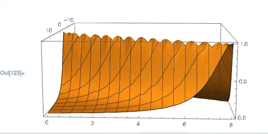
Walking witch
Often it is the case where a plug is moving through a pipe. This raises the question: what function to use to model a pulse?
Everyone likes polynomials, therefore, use the witch of Agnesi. In the instance where a=1/2 this simplifies the IC:
. Solve[2].

References
- Daileda, Ryan (January 2014). [ramanujan.math.trinity.edu/rdaileda/teach/s14/m3357/lectures/lecture_1_21_slides.pdf "Solving First Order PDEs"] Check
|url=value (help) (PDF). Trinity college. - "Partial Differential Equations (PDEs)—Wolfram Language Documentation". reference.wolfram.com. Retrieved 2021-02-01.
