Window function
In signal processing and statistics, a window function (also known as an apodization function or tapering function[1]) is a mathematical function that is zero-valued outside of some chosen interval, normally symmetric around the middle of the interval, usually near a maximum in the middle, and usually tapering away from the middle. Mathematically, when another function or waveform/data-sequence is "multiplied" by a window function, the product is also zero-valued outside the interval: all that is left is the part where they overlap, the "view through the window". Equivalently, and in actual practice, the segment of data within the window is first isolated, and then only that data is multiplied by the window function values. Thus, tapering, not segmentation, is the main purpose of window functions.
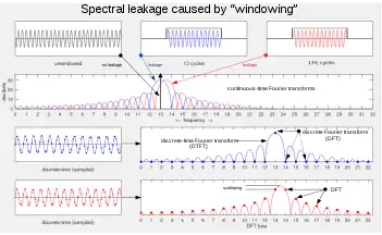
The reasons for examining segments of a longer function include detection of transient events and time-averaging of frequency spectra. The duration of the segments is determined in each application by requirements like time and frequency resolution. But that method also changes the frequency content of the signal by an effect called spectral leakage. Window functions allow us to distribute the leakage spectrally in different ways, according to the needs of the particular application. There are many choices detailed in this article, but many of the differences are so subtle as to be insignificant in practice.
In typical applications, the window functions used are non-negative, smooth, "bell-shaped" curves.[2] Rectangle, triangle, and other functions can also be used. A rectangular window does not modify the data segment at all. It's only for modelling purposes that we say it multiplies by 1 inside the window and by 0 outside. A more general definition of window functions does not require them to be identically zero outside an interval, as long as the product of the window multiplied by its argument is square integrable, and, more specifically, that the function goes sufficiently rapidly toward zero.[3]
Applications
Window functions are used in spectral analysis/modification/resynthesis,[4] the design of finite impulse response filters, as well as beamforming and antenna design.
Spectral analysis
The Fourier transform of the function cos(ωt) is zero, except at frequency ±ω. However, many other functions and waveforms do not have convenient closed-form transforms. Alternatively, one might be interested in their spectral content only during a certain time period.
In either case, the Fourier transform (or a similar transform) can be applied on one or more finite intervals of the waveform. In general, the transform is applied to the product of the waveform and a window function. Any window (including rectangular) affects the spectral estimate computed by this method.
Choice of window function
Windowing of a simple waveform like cos(ωt) causes its Fourier transform to develop non-zero values (commonly called spectral leakage) at frequencies other than ω. The leakage tends to be worst (highest) near ω and least at frequencies farthest from ω.
If the waveform under analysis comprises two sinusoids of different frequencies, leakage can interfere with our ability to distinguish them spectrally. Possible types of interference are often broken down into two opposing classes as follows: If the component frequencies are dissimilar and one component is weaker, then leakage from the stronger component can obscure the weaker one's presence. But if the frequencies are too similar, leakage can render them unresolvable even when the sinusoids are of equal strength. Windows that are effective against the first type of interference, namely where components have dissimilar frequencies and amplitudes, are called high dynamic range. Conversely, windows that can distinguish components with similar frequencies and amplitudes are called high resolution.
The rectangular window is an example of a window that is high resolution but low dynamic range, meaning it is good for distinguishing components of similar amplitude even when the frequencies are also close, but poor at distinguishing components of different amplitude even when the frequencies are far away. High-resolution, low-dynamic-range windows such as the rectangular window also have the property of high sensitivity, which is the ability to reveal relatively weak sinusoids in the presence of additive random noise. That is because the noise produces a stronger response with high-dynamic-range windows than with high-resolution windows.
At the other extreme of the range of window types are windows with high dynamic range but low resolution and sensitivity. High-dynamic-range windows are most often justified in wideband applications, where the spectrum being analyzed is expected to contain many different components of various amplitudes.
In between the extremes are moderate windows, such as Hamming and Hann. They are commonly used in narrowband applications, such as the spectrum of a telephone channel.
In summary, spectral analysis involves a trade-off between resolving comparable strength components with similar frequencies (high resolution / sensitivity) and resolving disparate strength components with dissimilar frequencies (high dynamic range). That trade-off occurs when the window function is chosen.[5]:p. 90
Discrete-time signals
When the input waveform is time-sampled, instead of continuous, the analysis is usually done by applying a window function and then a discrete Fourier transform (DFT). But the DFT provides only a sparse sampling of the actual discrete-time Fourier transform (DTFT) spectrum. Figure 2, row 3 shows a DTFT for a rectangularly-windowed sinusoid. The actual frequency of the sinusoid is indicated as "13" on the horizontal axis. Everything else is leakage, exaggerated by the use of a logarithmic presentation. The unit of frequency is "DFT bins"; that is, the integer values on the frequency axis correspond to the frequencies sampled by the DFT. So the figure depicts a case where the actual frequency of the sinusoid coincides with a DFT sample, and the maximum value of the spectrum is accurately measured by that sample. In row 4, it misses the maximum value by ½ bin, and the resultant measurement error is referred to as scalloping loss (inspired by the shape of the peak). For a known frequency, such as a musical note or a sinusoidal test signal, matching the frequency to a DFT bin can be prearranged by choices of a sampling rate and a window length that results in an integer number of cycles within the window.

Noise bandwidth
The concepts of resolution and dynamic range tend to be somewhat subjective, depending on what the user is actually trying to do. But they also tend to be highly correlated with the total leakage, which is quantifiable. It is usually expressed as an equivalent bandwidth, B. It can be thought of as redistributing the DTFT into a rectangular shape with height equal to the spectral maximum and width B.[upper-alpha 1][6] The more the leakage, the greater the bandwidth. It is sometimes called noise equivalent bandwidth or equivalent noise bandwidth, because it is proportional to the average power that will be registered by each DFT bin when the input signal contains a random noise component (or is just random noise). A graph of the power spectrum, averaged over time, typically reveals a flat noise floor, caused by this effect. The height of the noise floor is proportional to B. So two different window functions can produce different noise floors.
Processing gain and losses
In signal processing, operations are chosen to improve some aspect of quality of a signal by exploiting the differences between the signal and the corrupting influences. When the signal is a sinusoid corrupted by additive random noise, spectral analysis distributes the signal and noise components differently, often making it easier to detect the signal's presence or measure certain characteristics, such as amplitude and frequency. Effectively, the signal to noise ratio (SNR) is improved by distributing the noise uniformly, while concentrating most of the sinusoid's energy around one frequency. Processing gain is a term often used to describe an SNR improvement. The processing gain of spectral analysis depends on the window function, both its noise bandwidth (B) and its potential scalloping loss. These effects partially offset, because windows with the least scalloping naturally have the most leakage.
Figure 3 depicts the effects of three different window functions on the same data set, comprising two equal strength sinusoids in additive noise. The frequencies of the sinusoids are chosen such that one encounters no scalloping and the other encounters maximum scalloping. Both sinusoids suffer less SNR loss under the Hann window than under the Blackman–Harris window. In general (as mentioned earlier), this is a deterrent to using high-dynamic-range windows in low-dynamic-range applications.


Symmetry
The formulas provided in this article produce discrete sequences, as if a continuous window function has been "sampled". (See an example at Kaiser window.) Window sequences for spectral analysis are either symmetric or 1-sample short of symmetric (called periodic,[7][8] DFT-even, or DFT-symmetric[9]:p. 52). For instance, a true symmetric sequence, with its maximum at a single center-point, is generated by the MATLAB function hann(9,'symmetric'). Deleting the last sample produces a sequence identical to hann(8,'periodic'). Similarly, the sequence hann(8,'symmetric') has two equal center-points.[10]
Some functions have one or two zero-valued end-points, which are unnecessary in most applications. Deleting a zero-valued end-point has no effect on its DTFT (spectral leakage). But the function designed for N+1 or N+2 samples, in anticipation of deleting one or both end points, typically has a slightly narrower main lobe, slightly higher sidelobes, and a slightly smaller noise-bandwidth.[11]
DFT-symmetry
The predecessor of the DFT is the finite Fourier transform, and window functions were "always an odd number of points and exhibit even symmetry about the origin".[9]:p. 52 In that case, the DTFT is entirely real-valued. When the same sequence is shifted into a DFT data window, [0 ≤ n ≤ N], the DTFT becomes complex-valued, except at frequencies spaced at regular intervals of 1/N.[lower-alpha 1] Thus, when sampled by an N-length DFT (see periodic summation), the samples (called DFT coefficients) are still real-valued. Because of the periodic summation the last sample of the window function, w[N], is incorporated in the n = 0 term of the DFT: exp{−i2πk0/N} · (w[0] + w[N]) = w[0] + w[N], which is real-valued for all values of k (all DFT coefficients). So when the last sample of a symmetric sequence is truncated (w[N] = 0), the imaginary components remain zero.[upper-alpha 2] It does affect the DTFT (spectral leakage), but usually by a negligible amount (unless N is small, e.g. ≤ 20).[12][upper-alpha 3]
When windows are multiplicatively applied to actual data, the sequence usually lacks any symmetry, and the DFT is generally not real-valued. Despite this caveat, many authors reflexively assume DFT-symmetric windows.[9][13][14][15][16][17][lower-alpha 2] So it is worth noting that there is no performance advantage when applied to time domain data, which is the customary application. The advantage of real-valued DFT coefficients is realized in certain esoteric applications[upper-alpha 4] where windowing is achieved by means of convolution between the DFT coefficients and an unwindowed DFT of the data.[18][9]:p. 62[5]:p. 85 In those applications, DFT-symmetric windows (even or odd length) from the Cosine-sum family are preferred, because most of their DFT coefficients are zero-valued, making the convolution very efficient.[upper-alpha 5][5]:p. 85
Filter design
Windows are sometimes used in the design of digital filters, in particular to convert an "ideal" impulse response of infinite duration, such as a sinc function, to a finite impulse response (FIR) filter design. That is called the window method.[19][20][21]
Statistics and curve fitting
Window functions are sometimes used in the field of statistical analysis to restrict the set of data being analyzed to a range near a given point, with a weighting factor that diminishes the effect of points farther away from the portion of the curve being fit. In the field of Bayesian analysis and curve fitting, this is often referred to as the kernel.
Analysis of transients
When analyzing a transient signal in modal analysis, such as an impulse, a shock response, a sine burst, a chirp burst, or noise burst, where the energy vs time distribution is extremely uneven, the rectangular window may be most appropriate. For instance, when most of the energy is located at the beginning of the recording, a non-rectangular window attenuates most of the energy, degrading the signal-to-noise ratio.[22]
Harmonic analysis
One might wish to measure the harmonic content of a musical note from a particular instrument or the harmonic distortion of an amplifier at a given frequency. Referring again to Figure 2, we can observe that there is no leakage at a discrete set of harmonically-related frequencies sampled by the DFT. (The spectral nulls are actually zero-crossings, which cannot be shown on a logarithmic scale such as this.) This property is unique to the rectangular window, and it must be appropriately configured for the signal frequency, as described above.
A list of window functions
Conventions:
- is a zero-phase function (symmetrical about x = 0),[23] continuous for where N is a positive integer (even or odd).[24]
- The sequence is symmetric, of length
- is DFT-symmetric, of length [upper-alpha 6]


- The parameter B displayed on each spectral plot is the function's noise equivalent bandwidth metric, in units of DFT bins.
The sparse sampling of a DTFT (such as the DFTs in Fig 2) only reveals the leakage into the DFT bins from a sinusoid whose frequency is also an integer DFT bin. The unseen sidelobes reveal the leakage to expect from sinusoids at other frequencies.[lower-alpha 3] Therefore, when choosing a window function, it is usually important to sample the DTFT more densely (as we do throughout this section) and choose a window that suppresses the sidelobes to an acceptable level.
Rectangular window
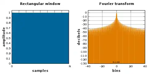
The rectangular window (sometimes known as the boxcar or Dirichlet window) is the simplest window, equivalent to replacing all but N values of a data sequence by zeros, making it appear as though the waveform suddenly turns on and off:

Other windows are designed to moderate these sudden changes, which reduces scalloping loss and improves dynamic range, as described above (§ Spectral analysis).
The rectangular window is the 1st order B-spline window as well as the 0th power power-of-sine window.
B-spline windows
B-spline windows can be obtained as k-fold convolutions of the rectangular window. They include the rectangular window itself (k = 1), the § Triangular window (k = 2) and the § Parzen window (k = 4).[25] Alternative definitions sample the appropriate normalized B-spline basis functions instead of convolving discrete-time windows. A kth order B-spline basis function is a piece-wise polynomial function of degree k−1 that is obtained by k-fold self-convolution of the rectangular function.
Triangular window
Triangular windows are given by:

where L can be N,[26] N + 1,[9] [27][28] or N + 2.[29] The first one is also known as Bartlett window or Fejér window. All three definitions converge at large N.
The triangular window is the 2nd order B-spline window. The L = N form can be seen as the convolution of two N/2-width rectangular windows. The Fourier transform of the result is the squared values of the transform of the half-width rectangular window.
Parzen window
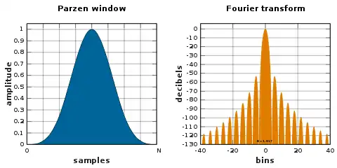
Defining L ≜ N + 1, the Parzen window, also known as the de la Vallée Poussin window,[9] is the 4th order B-spline window given by:


Welch window
The Welch window consists of a single parabolic section:

The defining quadratic polynomial reaches a value of zero at the samples just outside the span of the window.
Sine window
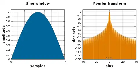

The corresponding function is a cosine without the π/2 phase offset. So the sine window[30] is sometimes also called cosine window.[9] As it represents half a cycle of a sinusoidal function, it is also known variably as half-sine window[31] or half-cosine window.[32]

The autocorrelation of a sine window produces a function known as the Bohman window.[33]
Power-of-sine/cosine windows
These window functions have the form:[34]

The rectangular window (α = 0), the sine window (α = 1), and the Hann window (α = 2) are members of this family.
Cosine-sum windows
This family is also known as generalized cosine windows.
-
(Eq.1)

In most cases, including the examples below, all coefficients ak ≥ 0. These windows have only 2K + 1 non-zero N-point DFT coefficients.
Hann and Hamming windows
.svg.png.webp)
The customary cosine-sum windows for case K = 1 have the form:

which is easily (and often) confused with its zero-phase version:

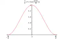
Setting produces a Hann window:


named after Julius von Hann, and sometimes referred to as Hanning, presumably due to its linguistic and formulaic similarities to the Hamming window. It is also known as raised cosine, because the zero-phase version, is one lobe of an elevated cosine function.

This function is a member of both the cosine-sum and power-of-sine families. Unlike the Hamming window, the end points of the Hann window just touch zero. The resulting side-lobes roll off at about 18 dB per octave.[35]
Setting to approximately 0.54, or more precisely 25/46, produces the Hamming window, proposed by Richard W. Hamming. That choice places a zero-crossing at frequency 5π/(N − 1), which cancels the first sidelobe of the Hann window, giving it a height of about one-fifth that of the Hann window.[9][36][37] The Hamming window is often called the Hamming blip when used for pulse shaping.[38][39][40]

Approximation of the coefficients to two decimal places substantially lowers the level of sidelobes,[9] to a nearly equiripple condition.[37] In the equiripple sense, the optimal values for the coefficients are a0 = 0.53836 and a1 = 0.46164.[37][5]
Hamming window is used for Audio Spectrum effect in Adobe After Effects.
Blackman window
Blackman windows are defined as:


By common convention, the unqualified term Blackman window refers to Blackman's "not very serious proposal" of α = 0.16 (a0 = 0.42, a1 = 0.5, a2 = 0.08), which closely approximates the exact Blackman,[41] with a0 = 7938/18608 ≈ 0.42659, a1 = 9240/18608 ≈ 0.49656, and a2 = 1430/18608 ≈ 0.076849.[42] These exact values place zeros at the third and fourth sidelobes,[9] but result in a discontinuity at the edges and a 6 dB/oct fall-off. The truncated coefficients do not null the sidelobes as well, but have an improved 18 dB/oct fall-off.[9][43]
Nuttall window, continuous first derivative
.svg.png.webp)
The continuous form of Nuttall window, and its first derivative are continuous everywhere, like the Hann function. That is, the function goes to 0 at x = ±N/2, unlike the Blackman–Nuttall, Blackman–Harris, and Hamming windows. The Blackman window (α = 0.16) is also continuous with continuous derivative at the edge, but the "exact Blackman window" is not.


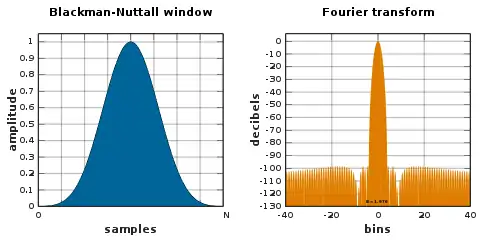
Blackman–Nuttall window

Blackman–Harris window
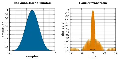
A generalization of the Hamming family, produced by adding more shifted sinc functions, meant to minimize side-lobe levels[44][45]

Flat top window

A flat top window is a partially negative-valued window that has minimal scalloping loss in the frequency domain. That property is desirable for the measurement of amplitudes of sinusoidal frequency components.[13][46] Drawbacks of the broad bandwidth are poor frequency resolution and high § Noise bandwidth.
Flat top windows can be designed using low-pass filter design methods,[46] or they may be of the usual cosine-sum variety:

The Matlab variant has these coefficients:

Other variations are available, such as sidelobes that roll off at the cost of higher values near the main lobe.[13]
Rife–Vincent windows
Rife–Vincent windows[47] are customarily scaled for unity average value, instead of unity peak value. The coefficient values below, applied to Eq.1, reflect that custom.
Class I, Order 1 (K = 1): Functionally equivalent to the Hann window.

Class I, Order 2 (K = 2):

Class I is defined by minimizing the high-order sidelobe amplitude. Coefficients for orders up to K=4 are tabulated.[48]
Class II minimizes the main-lobe width for a given maximum side-lobe.
Class III is a compromise for which order K = 2 resembles the § Blackman window.[48][49]
Gaussian window
.svg.png.webp)
The Fourier transform of a Gaussian is also a Gaussian. Since the support of a Gaussian function extends to infinity, it must either be truncated at the ends of the window, or itself windowed with another zero-ended window.[50]
Since the log of a Gaussian produces a parabola, this can be used for nearly exact quadratic interpolation in frequency estimation.[51][50][52]


The standard deviation of the Gaussian function is σ · N/2 sampling periods.
.svg.png.webp)
Confined Gaussian window
The confined Gaussian window yields the smallest possible root mean square frequency width σω for a given temporal width (N + 1) σt.[53] These windows optimize the RMS time-frequency bandwidth products. They are computed as the minimum eigenvectors of a parameter-dependent matrix. The confined Gaussian window family contains the § Sine window and the § Gaussian window in the limiting cases of large and small σt, respectively.
.svg.png.webp)
Approximate confined Gaussian window
Defining L ≜ N + 1, a confined Gaussian window of temporal width L × σt is well approximated by:[53]

where is a Gaussian function:


The standard deviation of the approximate window is asymptotically equal (i.e. large values of N) to L × σt for σt < 0.14.[53]
Generalized normal window
A more generalized version of the Gaussian window is the generalized normal window.[54] Retaining the notation from the Gaussian window above, we can represent this window as

for any even . At , this is a Gaussian window and as approaches , this approximates to a rectangular window. The Fourier transform of this window does not exist in a closed form for a general . However, it demonstrates the other benefits of being smooth, adjustable bandwidth. Like the § Tukey window, this window naturally offers a "flat top" to control the amplitude attenuation of a time-series (on which we don't have a control with Gaussian window). In essence, it offers a good (controllable) compromise, in terms of spectral leakage, frequency resolution and amplitude attenuation, between the Gaussian window and the rectangular window. See also [55] for a study on time-frequency representation of this window (or function).


Tukey window
.svg.png.webp)
The Tukey window, also known as the cosine-tapered window, can be regarded as a cosine lobe of width Nα/2 (spanning Nα/2+1 samples) that is convolved with a rectangular window of width N(1 − α/2).

At α = 0 it becomes rectangular, and at α = 1 it becomes a Hann window.
Planck-taper window
.svg.png.webp)
The so-called "Planck-taper" window is a bump function that has been widely used[57] in the theory of partitions of unity in manifolds. It is smooth (a function) everywhere, but is exactly zero outside of a compact region, exactly one over an interval within that region, and varies smoothly and monotonically between those limits. Its use as a window function in signal processing was first suggested in the context of gravitational-wave astronomy, inspired by the Planck distribution.[58] It is defined as a piecewise function:


The amount of tapering is controlled by the parameter ε, with smaller values giving sharper transitions.
DPSS or Slepian window
The DPSS (discrete prolate spheroidal sequence) or Slepian window maximizes the energy concentration in the main lobe,[59] and is used in multitaper spectral analysis, which averages out noise in the spectrum and reduces information loss at the edges of the window.
The main lobe ends at a frequency bin given by the parameter α.[60]
.svg.png.webp) DPSS window, α = 2 |
.svg.png.webp) DPSS window, α = 3 |
The Kaiser windows below are created by a simple approximation to the DPSS windows:
.svg.png.webp) Kaiser window, α = 2 |
.svg.png.webp) Kaiser window, α = 3 |
Kaiser window
The Kaiser, or Kaiser–Bessel, window is a simple approximation of the DPSS window using Bessel functions, discovered by James Kaiser.[61][62]
- [upper-alpha 9][9]:p. 73


where is the zero-th order modified Bessel function of the first kind. Variable parameter determines the tradeoff between main lobe width and side lobe levels of the spectral leakage pattern. The main lobe width, in between the nulls, is given by in units of DFT bins,[69] and a typical value of is 3.


Dolph–Chebyshev window
.svg.png.webp)
Minimizes the Chebyshev norm of the side-lobes for a given main lobe width.[70]
The zero-phase Dolph–Chebyshev window function is usually defined in terms of its real-valued discrete Fourier transform, :[71]


Tn(x) is the n-th Chebyshev polynomial of the first kind evaluated in x, which can be computed using

and

is the unique positive real solution to , where the parameter α sets the Chebyshev norm of the sidelobes to −20α decibels.[70]

The window function can be calculated from W0(k) by an inverse discrete Fourier transform (DFT):[70]

The lagged version of the window can be obtained by:

which for even values of N must be computed as follows:

which is an inverse DFT of

Variations:
- Due to the equiripple condition, the time-domain window has discontinuities at the edges. An approximation that avoids them, by allowing the equiripples to drop off at the edges, is a Taylor window.
- An alternative to the inverse DFT definition is also available..
Ultraspherical window
.svg.png.webp)
The Ultraspherical window was introduced in 1984 by Roy Streit[72] and has application in antenna array design,[73] non-recursive filter design,[72] and spectrum analysis.[74]
Like other adjustable windows, the Ultraspherical window has parameters that can be used to control its Fourier transform main-lobe width and relative side-lobe amplitude. Uncommon to other windows, it has an additional parameter which can be used to set the rate at which side-lobes decrease (or increase) in amplitude.[74][75]
The window can be expressed in the time-domain as follows:[74]

where is the Ultraspherical polynomial of degree N, and and control the side-lobe patterns.[74]


Certain specific values of yield other well-known windows: and give the Dolph–Chebyshev and Saramäki windows respectively.[72] See here for illustration of Ultraspherical windows with varied parametrization.


Exponential or Poisson window
.svg.png.webp)
.svg.png.webp)
The Poisson window, or more generically the exponential window increases exponentially towards the center of the window and decreases exponentially in the second half. Since the exponential function never reaches zero, the values of the window at its limits are non-zero (it can be seen as the multiplication of an exponential function by a rectangular window [76]). It is defined by

where τ is the time constant of the function. The exponential function decays as e ≃ 2.71828 or approximately 8.69 dB per time constant.[77] This means that for a targeted decay of D dB over half of the window length, the time constant τ is given by

Hybrid windows
Window functions have also been constructed as multiplicative or additive combinations of other windows.
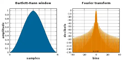
Bartlett–Hann window


Planck–Bessel window
.svg.png.webp)
A § Planck-taper window multiplied by a Kaiser window which is defined in terms of a modified Bessel function. This hybrid window function was introduced to decrease the peak side-lobe level of the Planck-taper window while still exploiting its good asymptotic decay.[78] It has two tunable parameters, ε from the Planck-taper and α from the Kaiser window, so it can be adjusted to fit the requirements of a given signal.
Hann–Poisson window
.svg.png.webp)
A Hann window multiplied by a Poisson window, which has no side-lobes, in the sense that its Fourier transform drops off forever away from the main lobe. It can thus be used in hill climbing algorithms like Newton's method.[79] The Hann–Poisson window is defined by:

where α is a parameter that controls the slope of the exponential.
Other windows
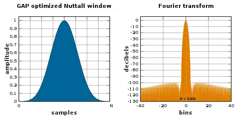
Generalized adaptive polynomial (GAP) window
The GAP window[80] is a family of adjustable window functions that are based on a symmetrical polynomial expansion of order . It is continuous with continuous derivative everywhere. With the appropriate set of expansion coefficients and expansion order, the GAP window can mimic all the known window functions, reproducing accurately their spectral properties.


where is the standard deviation of the sequence.


Additionally, starting with a set of expansion coefficients that mimics a certain known window function, the GAP window can be optimized by minimization procedures to get a new set of coefficients that improve one or more spectral properties, such as the main lobe width, side lobe attenuation, and side lobe falloff rate.[82] Therefore, a GAP window function can be developed with designed spectral properties depending on the specific application.

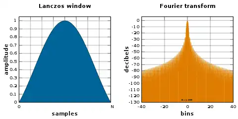
Lanczos window

- used in Lanczos resampling
- for the Lanczos window, is defined as
- also known as a sinc window, because:


- is the main lobe of a normalized sinc function

Comparison of windows

When selecting an appropriate window function for an application, this comparison graph may be useful. The frequency axis has units of FFT "bins" when the window of length N is applied to data and a transform of length N is computed. For instance, the value at frequency ½ "bin" (third tick mark) is the response that would be measured in bins k and k + 1 to a sinusoidal signal at frequency k + ½. It is relative to the maximum possible response, which occurs when the signal frequency is an integer number of bins. The value at frequency ½ is referred to as the maximum scalloping loss of the window, which is one metric used to compare windows. The rectangular window is noticeably worse than the others in terms of that metric.
Other metrics that can be seen are the width of the main lobe and the peak level of the sidelobes, which respectively determine the ability to resolve comparable strength signals and disparate strength signals. The rectangular window (for instance) is the best choice for the former and the worst choice for the latter. What cannot be seen from the graphs is that the rectangular window has the best noise bandwidth, which makes it a good candidate for detecting low-level sinusoids in an otherwise white noise environment. Interpolation techniques, such as zero-padding and frequency-shifting, are available to mitigate its potential scalloping loss.
Overlapping windows
When the length of a data set to be transformed is larger than necessary to provide the desired frequency resolution, a common practice is to subdivide it into smaller sets and window them individually. To mitigate the "loss" at the edges of the window, the individual sets may overlap in time. See Welch method of power spectral analysis and the modified discrete cosine transform.
Two-dimensional windows
Two-dimensional windows are commonly used in image processing to reduce unwanted high-frequencies in the image Fourier transform.[83] They can be constructed from one-dimensional windows in either of two forms.[84] The separable form, is trivial to compute. The radial form, , which involves the radius , is isotropic, independent on the orientation of the coordinate axes. Only the Gaussian function is both separable and isotropic.[85] The separable forms of all other window functions have corners that depend on the choice of the coordinate axes. The isotropy/anisotropy of a two-dimensional window function is shared by its two-dimensional Fourier transform. The difference between the separable and radial forms is akin to the result of diffraction from rectangular vs. circular appertures, which can be visualized in terms of the product of two sinc functions vs. an Airy function, respectively.


See also
Notes
- Mathematically, the noise equivalent bandwidth of transfer function H is the bandwidth of an ideal rectangular filter with the same peak gain as H that would pass the same power with white noise input. In the units of frequency f (e.g. hertz), it is given by:
- The terms DFT-even and periodic refer to the idea that if the truncated sequence were repeated periodically, it would be even-symmetric about n = 0, and its DTFT would be entirely real-valued.
- An example of the effect of truncation on spectral leakage is figure Gaussian windows. The graph labeled DTFT periodic8 is the DTFT of the truncated window labeled periodic DFT-even (both blue). The green graph labeled DTFT symmetric9 corresponds to the same window with its symmetry restored. The DTFT samples, labeled DFT8 periodic summation, are an example of using periodic summation to sample it at the same frequencies as the blue graph.
- Sometimes both a windowed and an unwindowed (rectangularly windowed) DFT are needed.
- For example, see figures DFT-even Hann window and Odd-length, DFT-even Hann window, which show that the N-point DFT of the sequence generated by hann(N,'periodic') has only three non-zero values. All the other samples coincide with zero-crossings of the DTFT.
- Some authors limit their attention to this important subset and to even values of N.[9][13] But the window coefficient formulas are still the ones presented here.
- This formula can be confirmed by simplifying the cosine function at MATLAB tukeywin and substituting r=α and x=n/N.
- Harris 1978 (p 67, eq 38) appears to have two errors: (1) The subtraction operator in the numerator of the cosine function should be addition. (2) The denominator contains a spurious factor of 2. Also, Fig 30 corresponds to α=0.25 using the Wikipedia formula, but to 0.75 using the Harris formula. Fig 32 is similarly mislabeled.
- The Kaiser window is often parametrized by β, where β = πα.[63][64] [65][66][60][67][19]:p. 474 The alternative use of just α facilitates comparisons to the DPSS windows.[68]

Page citations
- Harris 1978, p 52, where
- Nuttall 1981, p 85 (15a).
- Harris 1978, p 57, fig 10.

References
- Weisstein, Eric W. (2003). CRC Concise Encyclopedia of Mathematics. CRC Press. ISBN 978-1-58488-347-0.
- Roads, Curtis (2002). Microsound. MIT Press. ISBN 978-0-262-18215-7.
- Cattani, Carlo; Rushchitsky, Jeremiah (2007). Wavelet and Wave Analysis As Applied to Materials With Micro Or Nanostructure. World Scientific. ISBN 978-981-270-784-0.
-
"Overlap-Add (OLA) STFT Processing | Spectral Audio Signal Processing". www.dsprelated.com. Retrieved 2016-08-07.
The window is applied twice: once before the FFT (the "analysis window") and secondly after the inverse FFT prior to reconstruction by overlap-add (the so-called "synthesis window"). ... More generally, any positive COLA window can be split into an analysis and synthesis window pair by taking its square root.
- Nuttall, Albert H. (Feb 1981). "Some Windows with Very Good Sidelobe Behavior". IEEE Transactions on Acoustics, Speech, and Signal Processing. 29 (1): 84–91. doi:10.1109/TASSP.1981.1163506. Extends Harris' paper, covering all the window functions known at the time, along with key metric comparisons.
- Carlson, A. Bruce (1986). Communication Systems: An Introduction to Signals and Noise in Electrical Communication. McGraw-Hill. ISBN 978-0-07-009960-9.
- "Hann (Hanning) window - MATLAB hann". www.mathworks.com. Retrieved 2020-02-12.
- "Window Function". www.mathworks.com. Retrieved 2019-04-14.
- Harris, Fredric J. (Jan 1978). "On the use of Windows for Harmonic Analysis with the Discrete Fourier Transform" (PDF). Proceedings of the IEEE. 66 (1): 51–83. Bibcode:1978IEEEP..66...51H. CiteSeerX 10.1.1.649.9880. doi:10.1109/PROC.1978.10837. S2CID 426548. The fundamental 1978 paper on FFT windows by Harris, which specified many windows and introduced key metrics used to compare them.
- Robertson, Neil (18 December 2018). "Evaluate Window Functions for the Discrete Fourier Transform". DSPRelated.com. The Related Media Group. Retrieved 9 August 2020. Revised 22 February 2020.
- "Matlab for the Hann Window". ccrma.stanford.edu. Retrieved 2020-09-01.
-
Rohling, H.; Schuermann, J. (March 1983). "Discrete time window functions with arbitrarily low sidelobe level". Signal Processing. Forschungsinstitut Ulm, Sedanstr, Germany: AEG-Telefunken. 5 (2): 127–138. doi:10.1016/0165-1684(83)90019-1. Retrieved 8 August 2020.
It can be shown, that the DFT-even sampling technique as proposed by Harris is not the most suitable one.
- Heinzel, G.; Rüdiger, A.; Schilling, R. (2002). Spectrum and spectral density estimation by the Discrete Fourier transform (DFT), including a comprehensive list of window functions and some new flat-top windows (Technical report). Max Planck Institute (MPI) für Gravitationsphysik / Laser Interferometry & Gravitational Wave Astronomy. 395068.0. Retrieved 2013-02-10. Also available at https://pure.mpg.de/rest/items/item_152164_1/component/file_152163/content
- Lyons, Richard (1 June 1998). "Windowing Functions Improve FFT Results". EDN. Sunnyvale, CA: TRW. Retrieved 8 August 2020.
- Fulton, Trevor (4 March 2008). "DP Numeric Transform Toolbox". herschel.esac.esa.int. Herschel Data Processing. Retrieved 8 August 2020.
-
Poularikas, A.D. (1999). "7.3.1". In Poularikas, Alexander D. (ed.). The Handbook of Formulas and Tables for Signal Processing (PDF). Boca Raton: CRC Press LLC. ISBN 0849385792. Retrieved 8 August 2020.
Windows are even (about the origin) sequences with an odd number of points. The right-most point of the window will be discarded.
- Puckette, Miller (30 December 2006). "Fourier analysis of non-periodic signals". msp.ucsd.edu. UC San Diego. Retrieved 9 August 2020.
- US patent 6898235, Carlin, Joe; Terry Collins & Peter Hays et al., "Wideband communication intercept and direction finding device using hyperchannelization", published 1999-12-10, issued 2005-05-24, url2=https://worldwide.espacenet.com/patent/search/family/034590049/publication/US6898235B1?q=pn%3DUS6898235
- Oppenheim, Alan V.; Schafer, Ronald W.; Buck, John R. (1999). "7.2". Discrete-time signal processing (2nd ed.). Upper Saddle River, N.J.: Prentice Hall. pp. 465–478. ISBN 0-13-754920-2. url=https://d1.amobbs.com/bbs_upload782111/files_24/ourdev_523225.pdf
- "FIR Filters by Windowing – The Lab Book Pages". www.labbookpages.co.uk. Retrieved 2016-04-13.
- "Mastering Windows" (PDF). www.cg.tuwien.ac.at. Retrieved 2020-02-12.
- "The Fundamentals of Signal Analysis Application Note 243" (PDF). hpmemoryproject.org. Retrieved 10 April 2018.
- "Zero Phase Filters". ccrma.stanford.edu. Retrieved 2020-02-12.
- Rorabaugh, C.Britton (October 1998). DSP Primer. Primer series. McGraw-Hill Professional. p. 196. ISBN 978-0070540040.
- Toraichi, K.; Kamada, M.; Itahashi, S.; Mori, R. (1989). "Window functions represented by B-spline functions". IEEE Transactions on Acoustics, Speech, and Signal Processing. 37: 145–147. doi:10.1109/29.17517.
- "Bartlett Window". ccrma.stanford.edu. Retrieved 2016-04-13.
- Tukey, J.W. (1967). "An introduction to the calculations of numerical spectrum analysis". Spectral Analysis of Time Series: 25–46.
- "Triangular window – MATLAB triang". www.mathworks.com. Retrieved 2016-04-13.
- Welch, P. (1967). "The use of fast Fourier transform for the estimation of power spectra: A method based on time averaging over short, modified periodograms". IEEE Transactions on Audio and Electroacoustics. 15 (2): 70–73. Bibcode:1967ITAE...15...70W. doi:10.1109/TAU.1967.1161901.
- Bosi, Marina; Goldberg, Richard E. (2003). "Time to Frequency Mapping Part II: The MDCT". Introduction to Digital Audio Coding and Standards. The Springer International Series in Engineering and Computer Science. 721. Boston, MA: Springer US. p. 106. doi:10.1007/978-1-4615-0327-9. ISBN 978-1-4615-0327-9.
- Kido, Ken'iti; Suzuki, Hideo; Ono, Takahiko; Fukushima, Manabu (1998). "Deformation of impulse response estimates by time window in cross spectral technique". Journal of the Acoustical Society of Japan (E). 19 (5): 349–361. doi:10.1250/ast.19.349.
- Landisman, M.; Dziewonski, A.; Satô, Y. (1969-05-01). "Recent Improvements in the Analysis of Surface Wave Observations". Geophysical Journal International. 17 (4): 369–403. Bibcode:1969GeoJ...17..369L. doi:10.1111/j.1365-246X.1969.tb00246.x.
- "Bohman window – R2019B". www.mathworks.com. Retrieved 2020-02-12.
- "Power-of-Cosine Window Family". ccrma.stanford.edu. Retrieved 10 April 2018.
- "Hann or Hanning or Raised Cosine". ccrma.stanford.edu. Retrieved 2016-04-13.
- Enochson, Loren D.; Otnes, Robert K. (1968). Programming and Analysis for Digital Time Series Data. U.S. Dept. of Defense, Shock and Vibration Info. Center. p. 142.
- "Hamming Window". ccrma.stanford.edu. Retrieved 2016-04-13.
- "A digital quadrature amplitude modulation (QAM) Radio: Building a better radio" (PDF). users.wpi.edu. p. 28. Retrieved 2020-02-12.
- "Bits to Symbols to Signals and back again" (PDF). users.wpi.edu. p. 7. Retrieved 2020-02-12.
- Johnson, C.Richard, Jr; Sethares, William A.; Klein, Andrew G. (2011-08-18). "11". Software Receiver Design. Cambridge University Press. ISBN 978-1139501453. Also https://cnx.org/contents/QsVBJjB4@3.1:6R_ztzDY@4/Pulse-Shaping-and-Receive-Filtering
- Weisstein, Eric W. "Blackman Function". mathworld.wolfram.com. Retrieved 2016-04-13.
- "Characteristics of Different Smoothing Windows - NI LabVIEW 8.6 Help". zone.ni.com. Retrieved 2020-02-13.
- Blackman, R.B.; Tukey, J.W. (1959-01-01). The Measurement of Power Spectra from the Point of View of Communications Engineering. Dover Publications. p. 99. ISBN 9780486605074.
- "Blackman-Harris Window Family". ccrma.stanford.edu. Retrieved 2016-04-13.
- "Three-Term Blackman-Harris Window". ccrma.stanford.edu. Retrieved 2016-04-13.
- Smith, Steven W. (2011). The Scientist and Engineer's Guide to Digital Signal Processing. San Diego, California, USA: California Technical Publishing. Retrieved 2013-02-14.
- Rife, David C.; Vincent, G.A. (1970), "Use of the discrete Fourier transform in the measurement of frequencies and levels of tones", Bell Syst. Tech. J., 49 (2): 197–228, doi:10.1002/j.1538-7305.1970.tb01766.x
- Andria, Gregorio; Savino, Mario; Trotta, Amerigo (1989), "Windows and interpolation algorithms to improve electrical measurement accuracy", IEEE Transactions on Instrumentation and Measurement, 38 (4): 856–863, doi:10.1109/19.31004
- Schoukens, Joannes; Pintelon, Rik; Van Hamme, Hugo (1992), "The interpolated fast Fourier transform: a comparative study", IEEE Transactions on Instrumentation and Measurement, 41 (2): 226–232, doi:10.1109/19.137352
-
"Matlab for the Gaussian Window". ccrma.stanford.edu. Retrieved 2016-04-13.
Note that, on a dB scale, Gaussians are quadratic. This means that parabolic interpolation of a sampled Gaussian transform is exact. ... quadratic interpolation of spectral peaks may be more accurate on a log-magnitude scale (e.g., dB) than on a linear magnitude scale
- "Gaussian Window and Transform". ccrma.stanford.edu. Retrieved 2016-04-13.
- "Quadratic Interpolation of Spectral Peaks". ccrma.stanford.edu. Retrieved 2016-04-13.
- Starosielec, S.; Hägele, D. (2014). "Discrete-time windows with minimal RMS bandwidth for given RMS temporal width". Signal Processing. 102: 240–246. doi:10.1016/j.sigpro.2014.03.033.
- Chakraborty, Debejyo; Kovvali, Narayan (2013). "Generalized normal window for digital signal processing". 2013 IEEE International Conference on Acoustics, Speech and Signal Processing. pp. 6083–6087. doi:10.1109/ICASSP.2013.6638833. ISBN 978-1-4799-0356-6. S2CID 11779529.
- Diethorn, E.J. (1994). "The generalized exponential time-frequency distribution". IEEE Transactions on Signal Processing. 42 (5): 1028–1037. Bibcode:1994ITSP...42.1028D. doi:10.1109/78.295214.
- Bloomfield, P. (2000). Fourier Analysis of Time Series: An Introduction. New York: Wiley-Interscience.
- Tu, Loring W. (2008). "Bump Functions and Partitions of Unity". An Introduction to Manifolds. Universitext. New York: Springer. pp. 127–134. doi:10.1007/978-0-387-48101-2_13. ISBN 978-0-387-48098-5.
- McKechan, D.J.A.; Robinson, C.; Sathyaprakash, B.S. (21 April 2010). "A tapering window for time-domain templates and simulated signals in the detection of gravitational waves from coalescing compact binaries". Classical and Quantum Gravity. 27 (8): 084020. arXiv:1003.2939. Bibcode:2010CQGra..27h4020M. doi:10.1088/0264-9381/27/8/084020. S2CID 21488253.
- "Slepian or DPSS Window". ccrma.stanford.edu. Retrieved 2016-04-13.
- Smith, J.O. (2011). "Kaiser and DPSS Windows Compared". ccrma.stanford.edu. Retrieved 2016-04-13.
-
Kaiser, James F.; Kuo, Franklin F. (1966). System Analysis by Digital Computer. John Wiley and Sons. pp. 232–235.
This family of window functions was "discovered" by Kaiser in 1962 following a discussion with B. F. Logan of the Bell Telephone Laboratories. ... Another valuable property of this family ... is that they also approximate closely the prolate spheroidal wave functions of order zero.
- Kaiser, James F. (Nov 1964). "A family of window functions having nearly ideal properties". Unpublished Memorandum.
- Rabiner, Lawrence R.; Gold, Bernard (1975). "3.11". Theory and application of digital signal processing. Englewood Cliffs, N.J.: Prentice-Hall. p. 94. ISBN 0-13-914101-4.
- Crochiere, R.E.; Rabiner, L.R. (1983). "4.3.1". Multirate Digital Signal Processing. Englewood Cliffs, NJ: Prentice-Hall. p. 144. ISBN 0136051626.
- Lin, Yuan-Pei; Vaidyanathan, P.P. (June 1998). "A Kaiser Window Approach for the Design of Prototype Filters of Cosine Modulated Filterbanks" (PDF). IEEE Signal Processing Letters. 5 (6): 132–134. Bibcode:1998ISPL....5..132L. doi:10.1109/97.681427. S2CID 18159105. Retrieved 2017-03-16.
-
Smith, J.O. (2011). "Kaiser Window". ccrma.stanford.edu. Retrieved 2019-03-20.
Sometimes the Kaiser window is parametrized by α, where β = πα.
- "Kaiser Window, R2020a". www.mathworks.com. Mathworks. Retrieved 9 April 2020.
-
"Kaiser Window". www.dsprelated.com. Retrieved 2020-04-08.
The following Matlab comparison of the DPSS and Kaiser windows illustrates the interpretation of α as the bin number of the edge of the critically sampled window main lobe.
- Kaiser, James F.; Schafer, Ronald W. (1980). "On the use of the I0-sinh window for spectrum analysis". IEEE Transactions on Acoustics, Speech, and Signal Processing. 28: 105–107. doi:10.1109/TASSP.1980.1163349.
- "Dolph-Chebyshev Window". ccrma.stanford.edu. Retrieved 2016-04-13.
- "Dolph-Chebyshev Window Definition". ccrma.stanford.edu. Retrieved 2019-03-05.
- Kabal, Peter (2009). "Time Windows for Linear Prediction of Speech" (PDF). Technical Report, Dept. Elec. & Comp. Eng., McGill University (2a): 31. Retrieved 2 February 2014.
- Streit, Roy (1984). "A two-parameter family of weights for nonrecursive digital filters and antennas". Transactions of ASSP. 32: 108–118. doi:10.1109/tassp.1984.1164275.
- Deczky, Andrew (2001). "Unispherical Windows". ISCAS 2001. The 2001 IEEE International Symposium on Circuits and Systems (Cat. No.01CH37196). 2. pp. 85–88. doi:10.1109/iscas.2001.921012. ISBN 978-0-7803-6685-5. S2CID 38275201.
- Bergen, S.W.A.; Antoniou, A. (2004). "Design of Ultraspherical Window Functions with Prescribed Spectral Characteristics". EURASIP Journal on Applied Signal Processing. 2004 (13): 2053–2065. Bibcode:2004EJASP2004...63B. doi:10.1155/S1110865704403114.
- Smith, Julius O. III (2011-04-23). "Poisson Window". ccrma.stanford.edu. Retrieved 2020-02-12.
- Gade, Svend; Herlufsen, Henrik (1987). "Technical Review No 3-1987: Windows to FFT analysis (Part I)" (PDF). Brüel & Kjær. Retrieved 2011-11-22.
- Berry, C.P.L.; Gair, J.R. (12 December 2012). "Observing the Galaxy's massive black hole with gravitational wave bursts". Monthly Notices of the Royal Astronomical Society. 429 (1): 589–612. arXiv:1210.2778. Bibcode:2013MNRAS.429..589B. doi:10.1093/mnras/sts360. S2CID 118944979.
- "Hann-Poisson Window". ccrma.stanford.edu. Retrieved 2016-04-13.
- Justo, J. F.; Beccaro, W. (2020-10-26). "Generalized Adaptive Polynomial Window Function". IEEE Access. 8: 187584–187589. doi:10.1109/ACCESS.2020.3030903. S2CID 225050036. Retrieved 2020-10-31.
- Wesley Beccaro (2020-10-31), "Generalized Adaptive Polynomial Window Function", mathworks.com, retrieved 2020-11-02
- "Generalized Adaptive Polynomial Window Function". www.mathworks.com. Retrieved 2020-12-12.
- R. Hovden, Y. Jiang, H. Xin, L.F. Kourkoutis (2015). "Periodic Artifact Reduction in Fourier Transforms of Full Field Atomic Resolution Images". Microscopy and Microanalysis. 21 (2): 436–441. Bibcode:2015MiMic..21..436H. doi:10.1017/S1431927614014639. PMID 25597865.CS1 maint: multiple names: authors list (link)
- Bernstein, Matt A.; King, Kevin Franklin; Zhou, Xiaohong Joe (2004). Handbook of MRI Pulse Sequences. London: Elsevier Academic Press. pp. 495–499. ISBN 0120928612.
- Awad, A.I.; Baba, K. (2011). "An Application for Singular Point Location in Fingerprint Classification". Digital Information Processing and Communications. Communications in Computer and Information Science. 188. p. 262. doi:10.1007/978-3-642-22389-1_24. ISBN 978-3-642-22388-4.
Further reading
- Harris, Frederic J. (September 1976). "Windows, Harmonic Analysis, and the Discrete Fourier Transform" (PDF). apps.dtic.mil. Naval Undersea Center, San Diego. Retrieved 2019-04-08.
- Albrecht, Hans-Helge (2012). Tailored minimum sidelobe and minimum sidelobe cosine-sum windows. Version 1.0. ISBN 978-3-86918-281-0 ). editor: Physikalisch-Technische Bundesanstalt. Physikalisch-Technische Bundesanstalt. doi:10.7795/110.20121022aa. ISBN 978-3-86918-281-0.
- Bergen, S.W.A.; Antoniou, A. (2005). "Design of Nonrecursive Digital Filters Using the Ultraspherical Window Function". EURASIP Journal on Applied Signal Processing. 2005 (12): 1910–1922. Bibcode:2005EJASP2005...44B. doi:10.1155/ASP.2005.1910.
- Prabhu, K. M. M. (2014). Window Functions and Their Applications in Signal Processing. Boca Raton, FL: CRC Press. ISBN 978-1-4665-1583-3.
- US patent 7065150, Park, Young-Seo, "System and method for generating a root raised cosine orthogonal frequency division multiplexing (RRC OFDM) modulation", published 2003, issued 2006
External links
 Media related to Window function at Wikimedia Commons
- LabView Help, Characteristics of Smoothing Filters, http://zone.ni.com/reference/en-XX/help/371361B-01/lvanlsconcepts/char_smoothing_windows/
- Evaluation of Various Window Functions using Multi-Instrument
- Creation and properties of Cosine-sum Window functions, http://electronicsart.weebly.com/fftwindows.html
- Online Interactive FFT, Windows, Resolution, and Leakage Simulation | RITEC | Library & Tools
