C-squares
C-squares (acronym for the concise spatial query and representation system) is a system of spatially unique, location-based identifiers (geocodes) for areas on the surface of the earth, represented as cells from a latitude-longitude based Discrete Global Grid at a hierarchical set of resolution steps. The identifiers incorporate literal values of latitude and longitude in an interleaved notation (producing grid resolutions of 10, 1, 0.1 degrees, etc.), together with additional digits that support intermediate grid resolutions of 5, 0.5, 0.05 degrees, etc. The system was initially designed to represent data "footprints" or spatial extents in a more flexible manner than a standard minimum bounding rectangle, and to support "lightweight", text-based spatial querying; it can also provide a set of identifiers for grid cells used for assembly, storage and analysis of spatially organised data. Dataset extents expressed in c-squares notation can be visualised using a web-based utility, the c-squares mapper, an online instance of which is currently provided by CSIRO Oceans and Atmosphere in Australia. C-squares codes and associated published software are free to use and the software is released under version 2 of the GNU General Public License (GPL), a licence of the Free Software Foundation.
| Full name | Concise spatial query and representation system |
|---|---|
| Organisation | CSIRO |
| Introduced | 1 May 2002 |
| No. issued | resolution dependent, e.g.:
|
| No. of digits | resolution dependent, e.g.:
|
| Example |
|
| Website | csquares www |
History
The c-squares method was developed by Tony Rees at CSIRO Oceans and Atmosphere in Australia (then "CSIRO Marine Research") in 2001-2, initially as a method for spatial indexing, rapid query, and compact storage and visualization of dataset spatial "footprints" in an agency-specific metadata directory (data catalogue);[1] it was first publicly announced at the 2002 "EOGEO" Technical Workshop held at Ispra, Italy in May 2002.[2] A more complete description was published in the scientific literature in 2003, together with a web-accessible mapping utility entitled the "c-squares mapper" for visualisation of data extents expressed in the c-squares notation.[3] Since that time, a number of projects and international collaborations have employed c-squares to support spatial indexing and/or map production, including Fishbase (to map stored data points for any species), the Ocean Biogeographic Information System (OBIS),[4][5] AquaMaps,[6] data analysis to support the designation of marine biogeographic realms,[7] for multi-national fisheries data collation by the Scientific, Technical and Economic Committee for Fisheries (STECF) of the European Commission,[8] and for data reporting by ICES.[9][10] For its application in displaying and modelling global biodiversity data, c-squares was one of four components cited in the award of the Ebbe Nielsen Prize to Rees by the Global Biodiversity Information Facility (GBIF) in 2014.[11] The concept of representing dataset "footprints" as cells of spatial data of this nature and alignment was stated to have been inspired by the data addressing method in the U.S. National Oceanographic Data Center (NODC) "World Ocean Database" product,[12][1] which uses 10 degree World Meteorological Organization squares (the starting point for c-squares hierarchical subdivision) for organising its data content, and the set of 1:100,000 topographic maps issued by the national mapping agency for Australia (coverage and index here); each map covers a 0.5 degree square and, with its associated mapsheet labels, can notionally be used as a unit of spatial identification.[1] The method has been discussed further in texts on georeferencing, including those by Hill, 2006[13] and Guo et al., 2020;[14] unfortunately, in the latter account, a fundamental misconception is made regarding the nature of the method with the result that the system is presented as a single resolution of the Earth only, as undivided 10×10 degree squares.[15]
Rationale
Spatial data are inherently (at least) 2-dimensional; without additional indexing, a numeric range query in 2 dimensions (e.g. x and y, or latitude and longitude) is required to retrieve data items within a particular area. Such queries are computationally expensive so it can be beneficial to pre-process (index) the data in some manner that reduces the inherent dimensionality from two to one dimension, for example as labelled cells of a grid. The grid labels can then be indexed by standard, one dimensional methods for rapid search and retrieval,[16] and/or searched by simple alphanumeric text searches. C-squares is an example of such a grid where the cell identifiers are designed to be human- as well as machine-readable, and to be concordant with recognizable and commonly intervals of latitude and longitude.
Additional areas where a grid-based approach to spatial indexing can be beneficial can be for the representation of data "footprints" in support of spatial search,[13] data binning to reduce complex and potentially voluminous data into "blocks" which then can be more easily compared and summarised, and the potential for a hierarchical approach wherein finer resolutions of the grid are nested into coarser ones, with a shared notation (common identifiers for the larger portions of the relevant grid cells). A jurisdiction-independent, (global) grid such as c-squares can also be used to integrate data across national boundaries, in contrast to (for example) the national grids of various countries such as those of the United Kingdom, Ireland, etc., which are not the same in their approach and may have differences or gaps where such grids overlap, or fail to meet (for example in marine regions around two areas).
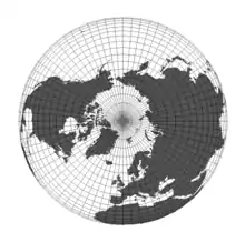
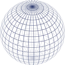
A potential disadvantage of "equal angle" grids (the class that includes c-squares), which are based on standardised units of latitude and longitude, is that the length of the "sides" and the shape (and area) of the grid cells is not constant on the ground (the height remains approximately constant but the width varies with latitude), and some particular effects are noticeable at the poles, where the cells become 3- rather than 4-sided in practice (refer illustration). These disadvantages can be offset by the advantages that data transformation in and out of grid notation can be accomplished by relatively straightforward steps, the results are congruent with conventional maps that show intervals of latitude and longitude, and the concepts of (for example) "1-degree squares" and "0.5 degree squares" may have familiarity and meaning to human users, in a way that non-square, purely mathematically derived shapes and sizes (based upon some form of spherical trigonometry) may not.
The c-squares global grid notation
Initial 10 degree squares
10-degree c-squares are specified as being identical to equivalent World Meteteorological Organization (WMO) square codes, refer illustration at right. These squares are aligned with 10-degree subdivisions of the global latitude–longitude grid, which for c-squares use is specified as employing the WGS84 datum. WMO (10 degree) squares are encoded with four digits, in the series 1xxx, 3xxx, 5xxx and 7xxx.[12] The leading digit indicates the "global quadrant" with 1 for north-east (latitude and longitude are both positive), 3 for south-east (latitude is negative and longitude positive), 5 for south-west (latitude and longitude are both negative) and 7 for north-west (latitude is positive and longitude negative). The next digit, 0 through 8, corresponds to the tens of latitude degrees either north or south; while the remaining 2 digits, 00 through 17, correspond to the tens of longitude degrees either east or west (by specification, 0 is treated as positive). Thus the 10 degree cell with its lower left corner at 0,0 (latitude,longitude) is encoded 1000, and acts as a bin to contain all spatial data between 0 and 10 degrees north (actually, 0 and 9.999...) and 0 and 9.999... degrees east; the 10 degree cell with its lower left corner at 80 N, 170 E is encoded 1817, and acts as a bin to contain all spatial data between 80 and 90 degrees north and 170 and 179.999... degrees east.
Subsequent recursive subdivision
C-squares extends the initial WMO 10×10 square notation via a recursive series of "cycles", each 3 digits long (the final one may be 1 digit), separated by the colon character, the number of characters (and cycles) indicating the resolution encoded, as per these examples:
- 1000 ... 10×10 degree square (up to 1000×1000 km nominal)
- 1000:1 ... 5×5 degree square (up to 500×500 km nominal)
- 1000:100 ... 1×1 degree square (up to 100×100 km nominal)
- 1000:100:1 ... 0.5×0.5 degree square (up to 50×50km nominal)
- 1000:100:100 ... 0.1×0.1 degree square (up to 10×10 km nominal)
- 1000:100:100:1 ... 0.05×0.05 degree square (up to 5×5km nominal)
(etc.)
Cell size is typically selected to suit the nature (granularity and volume) of the data to be encoded, the overall spatial extent of the area in question (e.g. global to local), the desired spatial resolution of the resulting grid (smallest features/areas that can be differentiated from each other), and the computing resources available (numbers of cells to cover the same area increase by either ×4 or ×25 with each decrease in square size, either requiring an equivalent increase in computing resources or possibly slower addressing times). For example, relatively generalised, global compilations may be best suited to aggregate (index) data by 10- or 5- degree cells, while more local gridded areas may favour 1-, 0.5- or 0.1- degree cells, as appropriate.
The nominal sizes given above reflect the fact that at the equator, 1 degree of both latitude and longitude correspond to around 110 km, with the actual value for longitude declining between there and the poles, where it becomes zero (latitude actual: 110.567 km at the equator, 111.699 km at the poles; longitude actual: 111.320 km at the equator, 78.847 km at latitude ±45 degrees, 0 km at the poles); at a sample northern hemisphere latitude e.g. that of London (51.5 degrees north), a 1×1 degree square measures approximately 111×69 km.[17]
To produce the 1 or 3 digits in any cycle following the initial 4-digit, 10-degree square identifier, first an "intermediate quadrant", 1 through 4 is designated (refer diagram at right), where 1 indicates low absolute values of both latitude and longitude (regardless of sign), 2 indicates low longitude and high latitude, 3 indicates high latitude and low longitude, and 4 indicates high values for both; "low" and high" being taken from the relevant portion of the data to be gridded (for example within the 10 degree cell extending from 10 to 20 degrees, 10 is treated as low and 19 as high). This leading digit in a cycle is then followed simply by the next applicable digit for first latitude and then longitude: thus an input value of latitude +11.0, longitude +12.0 degrees will be encoded as the 5 degree c-square code 1101:1 and the 1 degree code 1101:112. Inspection of this code will show that the input latitude value can be recovered directly from the digits 1101:112 while the longitude is included as 1101:112; the sign for these is both positive, as indicated by the first digit of the leading 4 (1 in this case, indicating the north east global quadrant).
From 2002 onwards (still current at 2020), an online "latlong to c-squares conversion page" is available at the website of CSIRO Marine Research (now CSIRO Oceans and Atmosphere) which will convert input values of latitude and longitude to the equivalent c-square code at user selectable resolutions from 10 to 0.1 degree cell size. Alternatively it is a comparatively simple task to program from first principles (or construct as, for example, a Microsoft Excel worksheet) according to the c-squares specification;[18] an example is available here.
C-squares strings, and the c-squares mapper
A set of c-squares (contiguous or non contiguous) can be represented as a concatenated list of individual square codes, separated by the "pipe" (|) character, thus: 7500:110:3|7500:110:1|1500:110:3|1500:110:1 (etc.). This set of squares can then serve as an indication of a dataset extent, similar in function (but simpler to specify) to a MultiPolygon in the Well-known text representation of geometry, the functional difference being that defined points forming the boundary of a polygon can be continuously variable, while those for the c-square boundaries are constrained to fixed intervals from the grid square resolution in use. If these strings are stored, for example as "long text" within a field of a conventional text storage system (e.g. spreadsheet, database, etc.) they can be used for the operation of spatial searches (see following section/s).
C-squares strings can also be used directly as input to an instance of the "c-squares mapper", a web-based utility in operation since 2002 at CSIRO in Australia (under the domain obis.org.au) and also at other global locations. To visualize the position of any set of squares on a map, the current syntax to address an installation of the "c-squares mapper" is (e.g.):
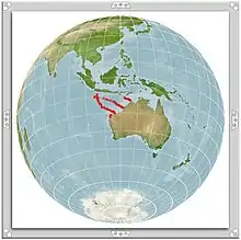
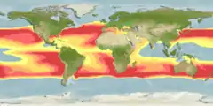
It should be noted here that the above call to the c-squares mapper is a simple one, with only a single parameter (a single c-squares string) which produces a simple "default map"; the mapper is in fact quite highly customizable, capable of accepting up to seven c-squares strings concurrently, plotting them in user-specified colours, with a choice of empty of filled squares, user-selectable base map, etc. etc.; a full list of available input parameters is provided on the mapper "technical information" page.[19] A more sophisticated map produced using a larger number of available parameters is the colour-coded example at right (AquaMap, i.e. modelled distribution, for the ocean sunfish). Commencing in 2006, an upgrade of the mapper incorporating the independently-written Xplanet software also allows the plots of supplied c-squares to be displayed on a user-rotatable and zoomable globe, which can offer a more realistic view for either Pacific Ocean- or polar- centred data than are possible with a flat map (e.g. equirectangular) projection.[20]
Spatial searching
In a system that uses c-squares codes as units of spatial indexing, a text-based search on any of these square identifiers will retrieve data associated with the relevant square. If a wildcard search is supported (for example in the case that the wildcard character is a percent sign), a search on "7500%" will retrieve all data items in that ten degree square, a search on "7500:1%" will retrieve all data items in that five degree square, etc.
The asterisk character "*" has a special (reserved) meaning in c-squares notation, being a "compact" notation indicating that all finer cells within a higher level cell are included, to the level of resolution indicated by the number of asterisks. In the example above, "7500:*" would indicate that all 4 five-degree cells within parent ten-degree cell "7500" are filled, "7500:***" would indicate that all 100 one-degree cells within parent ten-degree cell "7500" are filled, etc. This approach enables the filling of contiguous blocks of cells with an economy of characters in many cases (a form of data compression), that is useful for efficient storage and transfer of c-squares codes as required.
Spatial data reporting, assembly, and analysis
Examples of the use of c-squares for (sometimes multi-national) data reporting, assembly and analysis include the use of 0.05×0.05 degree c-squares for VMS (vessel monitoring systems) data and fishing logbook data for ICES, the International Council for the Exploration of the Sea and others,[10][21][22] identification of vulnerable marine ecosystems in the North-East Atlantic,[23] the use of 0.1×0.1 degree c-squares for fish catch reporting for the purpose of stock assessment in Australia,[24] the reporting and collation of fishing activity by member states into 0.5×0.5 degree c-squares by the Scientific, Technical and Economic Committee for Fisheries (STECF) of the European Commission,[8][25] and the use of squares of the same resolution for analysing and forecasting fisheries time series data in the Indian Ocean[26] and for delineating high priority areas for marine biodiversity conservation in the Coral Triangle, bordered by both the Pacific and Indian Oceans.[27] The marine species distribution modelling project "AquaMaps" makes available its base data coverages of global marine environmental variables as c-squares gridded data at 0.5 degree resolution,[28] while production of the first world scale map of marine biogeographic realms based on distributions of 65,000 marine species, by Costello et al., 2017, employed 5×5 degree squares (500×500 km nominal).[7]
Target audience/potential users
According to its design principles, the principal target audience for c-squares is data custodians who wish to organise spatial data by latitude-longitude grid squares at any of the resolutions supported by the system, namely any decimal subdivision of either 10×10 or 5×5 degree squares, to support associated data query, retrieval, analysis, representation (mapping), and potential external data exchange and aggregation. Fine resolution c-squares may also be used as a general "location encoder", selected desirable attributes of which are discussed further by the developers of the Google Open Location Code method,[29] since the c-squares method satisfies the majority of the criteria set out in that discussion document. As evidenced by the references cited in this article, principal adopters of the method to date have been concerned with marine data in particular; this most likely stems from the fact that the oceans are trans-national in their governance, therefore otherwise established local or national grids are unsuitable for analysis of ocean or fisheries data on anything other than a local scale, and also possibly from a perception that the system is targeted towards oceanographic data as per its initial deployment in marine-related systems plus its description in the journal "Oceanography"; nevertheless, in essence the system is terrain-agnostic (as is the latitude-longitude grid upon which it is based) and is applicable equally to both marine and terrestrial data.
Licensing and software availability
There is no licence required to use the c-squares method, which has been openly published in the scientific literature since 2003. Source code for the mapper, etc., available via the SourceForge website, is released under the GNU General Public License version 2.0 (GPLv2), which provides free use and redistribution, and subsequent modification for any purpose so long as that licence is retained with the product and any subsequent modifications, in other words, that all the released improved versions will also be free software.[30]
See also
References
- CSIRO Marine Research, 2002: About C-Squares.
- Rees, Tony (2002): "C-squares–a new metadata element for improved spatial querying and representation of spatial dataset coverage in metadata records" [abstract]. Proceedings of EOGEO Technical Workshop May 2002, Ispra, Italy. Archived copy available via the Internet Archive (accessed 24 October 2020)
- Rees, Tony (2003). "'C-squares', a new spatial indexing system and its applicability to the description of oceanographic datasets". Oceanography. 16 (1): 11–19. doi:10.5670/oceanog.2003.52.
- Tony Rees and Phoebe Zhang, 2007. "Evolving concepts in the architecture and functionality of OBIS, the Ocean Biogeographic Information System". in Vanden Berghe, E. et al. (ed.) Proceedings of Ocean Biodiversity Informatics: an international conference on marine biodiversity data management Hamburg, Germany, 29 November-1 December, 2004. IOC Workshop Report, 202, VLIZ Special Publication 37: pp. 167-176.
- Fujioka, Ei; Vanden Berghe, Edward; Donnelly, Ben; et al. (2012). "Advancing global marine biogeography research with open-source GIS software and cloud computing". Transactions in GIS. 16 (2): 143–160. doi:10.1111/j.1467-9671.2012.01310.x.
- Ready, Jonathan; Kaschner, Kristin; South, Andy B.; et al. (2010). "Predicting the distributions of marine organisms at the global scale". Ecological Modelling. 221 (3): 467–478. doi:10.1016/j.ecolmodel.2009.10.025.
- Costello, Mark J.; Tsai, Peter; Wong, Pui Shan; Cheung, Alan Kwok Lun; Basher, Zeenatul; Chaudhary, Chhaya (2017). "Marine biogeographic realms and species endemicity". Nature Communications. 8 (3): article 1057. doi:10.1038/s41467-017-01121-2. PMC 5648874. PMID 29051522.
- Willy Vanhee, Arina Motova & Antonella Zanzi (eds) (2018). Scientific, Technical and Economic Committee for Fisheries - 59th Plenary Meeting Report (PLEN-18-03). Publications Office of the European Union, Luxembourg, 95 pp. ISBN 978-92-79-98374-0, doi:10.2760/335280
- ICES, 2011. Report of the Study Group on VMS data, its storage, access and tools for analysis (SGVMS), 7–9 September 2011, Hamburg, Germany. ICES CM 2011/SSGSUE:07. 27 pp. Available online at http://www.ices.dk/sites/pub/Publication%20Reports/Expert%20Group%20Report/SSGSUE/2011/SGVMS11.pdf
- International Council for the Exploration of the Sea (2019) ICES Technical Guidelines: 16.3.3.3 Spatial distribution of fishing effort and physical disturbance of benthic habitats by mobile bottom trawl fishing gear using VMS. doi: 10.17895/ices.advice.4683 1 Available at https://www.ices.dk/sites/pub/Publication%20Reports/Guidelines%20and%20Policies/16.03.03.03_Guidelines_Vessel_Monitoring_Systems_Data.pdf
- gbif.org, News, 13 July 2014: CSIRO’s Tony Rees named 2014 Ebbe Nielsen Prize winner
- U.S. National Oceanographic Data Centre, 1998: "World Ocean Database 1998: Documentation and Quality Control, Version 1.2." Appendix 10A: World Meteorological Organization (WMO) Squares for the Atlantic and Indian Oceans; Appendix 10B: World Meteorological Organization (WMO) Squares for the Pacific Ocean.
- Hill, Linda (2006). Georeferencing: The Geographic Associations of Information. MIT Press, Cambridge, Mass. and London, England, 260 pp. ISBN 978-0-262-08354-6
- Huadong Guo, Michael F. Goodchild & Alessandro Annoni (eds.) (2020). Manual of Digital Earth. Springer, Singapore, 852 pp. ISBN 978-981-32-9914-6
- Chapter 2, "Digital Earth Platforms" by Troy Alderson et al., in Guo et al. (2020), p.43.
- Rigaux, P., Scholl, M., and Voisard, A. 2002. Spatial Databases - with application to GIS. Morgan Kaufmann, San Francisco, 410pp.
- U.S. National Hurricane Center and Central Pacific Hurricane Center: Latitude/Longitude Distance Calculator
- C-squares Specification - Version 1.1 (December 2005)
- CMAR c-squares Mapper - Technical Information page
- obis.org.au: C-squares mapper help. Accessed 7 December 2020.
- Hintzen, Niels T.; Bastardie, Francois; Beare, Doug; Piet, Gerjan J.; Ulrich, Clara; Deporte, Nicolas; Egekvist, Josefine; Degel, Henrik (2012). "VMStools: Open-source software for the processing, analysis and visualisation of fisheries logbook and VMS data". Fisheries Research. 115–116: 31–43. doi:10.1016/j.fishres.2011.11.007.
- Schulte, K. F.; Siegel, V.; Hufnagl, M.; Schulze, M.; Temming, A. (2020). "Spatial and temporal distribution patterns of brown shrimp (Crangon crangon) derived from commercial logbook, landings, and vessel monitoring data". ICES Journal of Marine Science. 77 (3): 1017–1032. doi:10.1093/icesjms/fsaa021.
- Morato, Telmo; Pham, Christopher K.; Pinto, Carlos; Golding, Neil; Ardron, Jeff A.; Muñoz, Pablo Durán; Neat, Francis (2018). "A multi criteria assessment method for identifying vulnerable marine ecosystems in the North-East Atlantic". Frontiers in Marine Science. 5: 460. doi:10.3389/fmars.2018.00460.
- Hall, K.C. (2020). Stock assessment report 2019 – Ocean Trawl Fishery – Bluespotted Flathead (Platycephalus caeruleopunctatus). NSW Department of Primary Industries, Coffs Harbour, 67 pp.
- Holmes, S.J., Gibin, M., Scott, F., Zanzi, A., et al. (2018). Report on the STECF Expert Working Group 17-12 Fisheries Dependent Information: 'New-FDI', EUR 29204 EN, European Union, Luxembourg. ISBN 978-92-79-85241-1, doi:10.2760/094412. Available at https://publications.jrc.ec.europa.eu/repository/bitstream/JRC111443/jrc_technical_report_stecf-17-12_new-fdi_final_1.pdf
- Coro, Gianpaolo; Large, Scott; Magliozzi, Chiara; Pagano, Pasquale (2016). "Analysing and forecasting fisheries time series: purse seine in Indian Ocean as a case study". ICES Journal of Marine Science. 73 (10): 2552–2571. doi:10.1093/icesjms/fsw131.
- Asaad, Irawan; Lundquist, Carolyn J.; Erdmann, Mark V.; Costello, Mark J. (2018). "Delineating priority areas for marine biodiversity conservation in the Coral Triangle". Biological Conservation. 222: 198–211. doi:10.1016/j.biocon.2018.03.037.
- Kesner-Reyes, K., Segschneider, J., Garilao, C., Schneider, B., Rius-Barile, J., Kaschner, K. and Froese, R. (editors). AquaMaps Environmental Dataset: Half-Degree Cells Authority File (HCAF). World Wide Web electronic publication, www.aquamaps.org/main/envt_data.php, ver. 7, 10/2019. (announced; previous versions available for download via https://www.aquamaps.org/main/envt_data.php)
- Anonymous, 2014-2018: "An Evaluation of Location Encoding Systems". Available from github.com/google/open-location-code (accessed 24 October 2020)
- Free Software Foundation: Frequently Asked Questions about version 2 of the GNU GPL
External links
- C-squares home page
- C-squares project page on SourceForge, including:
- lists of c-squares by ID, at resolutions from 10×10 to 0.5×0.5 degrees
- ESRI shapefiles containing equivalent information
- AquaMaps (demonstration of c-squares in real-world use)
