Kernel method
In machine learning, kernel machines are a class of algorithms for pattern analysis, whose best known member is the support vector machine (SVM). The general task of pattern analysis is to find and study general types of relations (for example clusters, rankings, principal components, correlations, classifications) in datasets. For many algorithms that solve these tasks, the data in raw representation have to be explicitly transformed into feature vector representations via a user-specified feature map: in contrast, kernel methods require only a user-specified kernel, i.e., a similarity function over pairs of data points in raw representation.
| Part of a series on |
| Machine learning and data mining |
|---|
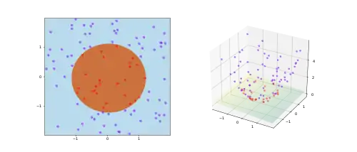
Kernel methods owe their name to the use of kernel functions, which enable them to operate in a high-dimensional, implicit feature space without ever computing the coordinates of the data in that space, but rather by simply computing the inner products between the images of all pairs of data in the feature space. This operation is often computationally cheaper than the explicit computation of the coordinates. This approach is called the "kernel trick".[1] Kernel functions have been introduced for sequence data, graphs, text, images, as well as vectors.
Algorithms capable of operating with kernels include the kernel perceptron, support vector machines (SVM), Gaussian processes, principal components analysis (PCA), canonical correlation analysis, ridge regression, spectral clustering, linear adaptive filters and many others. Any linear model can be turned into a non-linear model by applying the kernel trick to the model: replacing its features (predictors) by a kernel function.
Most kernel algorithms are based on convex optimization or eigenproblems and are statistically well-founded. Typically, their statistical properties are analyzed using statistical learning theory (for example, using Rademacher complexity).
Motivation and informal explanation
Kernel methods can be thought of as instance-based learners: rather than learning some fixed set of parameters corresponding to the features of their inputs, they instead "remember" the -th training example and learn for it a corresponding weight . Prediction for unlabeled inputs, i.e., those not in the training set, is treated by the application of a similarity function , called a kernel, between the unlabeled input and each of the training inputs . For instance, a kernelized binary classifier typically computes a weighted sum of similarities
- ,
where
- is the kernelized binary classifier's predicted label for the unlabeled input whose hidden true label is of interest;
- is the kernel function that measures similarity between any pair of inputs ;
- the sum ranges over the n labeled examples in the classifier's training set, with ;
- the are the weights for the training examples, as determined by the learning algorithm;
- the sign function determines whether the predicted classification comes out positive or negative.
Kernel classifiers were described as early as the 1960s, with the invention of the kernel perceptron.[2] They rose to great prominence with the popularity of the support vector machine (SVM) in the 1990s, when the SVM was found to be competitive with neural networks on tasks such as handwriting recognition.
Mathematics: the kernel trick

The kernel trick avoids the explicit mapping that is needed to get linear learning algorithms to learn a nonlinear function or decision boundary. For all and in the input space , certain functions can be expressed as an inner product in another space . The function is often referred to as a kernel or a kernel function. The word "kernel" is used in mathematics to denote a weighting function for a weighted sum or integral.
Certain problems in machine learning have more structure than an arbitrary weighting function . The computation is made much simpler if the kernel can be written in the form of a "feature map" which satisfies
The key restriction is that must be a proper inner product. On the other hand, an explicit representation for is not necessary, as long as is an inner product space. The alternative follows from Mercer's theorem: an implicitly defined function exists whenever the space can be equipped with a suitable measure ensuring the function satisfies Mercer's condition.
Mercer's theorem is similar to a generalization of the result from linear algebra that associates an inner product to any positive-definite matrix. In fact, Mercer's condition can be reduced to this simpler case. If we choose as our measure the counting measure for all , which counts the number of points inside the set , then the integral in Mercer's theorem reduces to a summation
If this summation holds for all finite sequences of points in and all choices of real-valued coefficients (cf. positive definite kernel), then the function satisfies Mercer's condition.
Some algorithms that depend on arbitrary relationships in the native space would, in fact, have a linear interpretation in a different setting: the range space of . The linear interpretation gives us insight about the algorithm. Furthermore, there is often no need to compute directly during computation, as is the case with support vector machines. Some cite this running time shortcut as the primary benefit. Researchers also use it to justify the meanings and properties of existing algorithms.
Theoretically, a Gram matrix with respect to (sometimes also called a "kernel matrix"[3]), where , must be positive semi-definite (PSD).[4] Empirically, for machine learning heuristics, choices of a function that do not satisfy Mercer's condition may still perform reasonably if at least approximates the intuitive idea of similarity.[5] Regardless of whether is a Mercer kernel, may still be referred to as a "kernel".
If the kernel function is also a covariance function as used in Gaussian processes, then the Gram matrix can also be called a covariance matrix.[6]
Applications
Application areas of kernel methods are diverse and include geostatistics,[7] kriging, inverse distance weighting, 3D reconstruction, bioinformatics, chemoinformatics, information extraction and handwriting recognition.
Popular kernels
References
- Theodoridis, Sergios (2008). Pattern Recognition. Elsevier B.V. p. 203. ISBN 9780080949123.
- Aizerman, M. A.; Braverman, Emmanuel M.; Rozonoer, L. I. (1964). "Theoretical foundations of the potential function method in pattern recognition learning". Automation and Remote Control. 25: 821–837. Cited in Guyon, Isabelle; Boser, B.; Vapnik, Vladimir (1993). Automatic capacity tuning of very large VC-dimension classifiers. Advances in neural information processing systems. CiteSeerX 10.1.1.17.7215.
- Hofmann, Thomas; Scholkopf, Bernhard; Smola, Alexander J. (2008). "Kernel Methods in Machine Learning". Cite journal requires
|journal=(help) - Mohri, Mehryar; Rostamizadeh, Afshin; Talwalkar, Ameet (2012). Foundations of Machine Learning. USA, Massachusetts: MIT Press. ISBN 9780262018258.
- Sewell, Martin. "Support Vector Machines: Mercer's Condition". www.svms.org.
- Rasmussen, C. E.; Williams, C. K. I. (2006). "Gaussian Processes for Machine Learning". Cite journal requires
|journal=(help) - Honarkhah, M.; Caers, J. (2010). "Stochastic Simulation of Patterns Using Distance-Based Pattern Modeling". Mathematical Geosciences. 42: 487–517. doi:10.1007/s11004-010-9276-7.
Further reading
- Shawe-Taylor, J.; Cristianini, N. (2004). Kernel Methods for Pattern Analysis. Cambridge University Press.
- Liu, W.; Principe, J.; Haykin, S. (2010). Kernel Adaptive Filtering: A Comprehensive Introduction. Wiley.
- Schölkopf, B.; Smola, A. J.; Bach, F. (2018). Learning with Kernels : Support Vector Machines, Regularization, Optimization, and Beyond. MIT Press. ISBN 978-0-262-53657-8.
External links
- Kernel-Machines Org—community website
- www.support-vector-machines.org (Literature, Review, Software, Links related to Support Vector Machines - Academic Site)
- onlineprediction.net Kernel Methods Article
