Lorenz system
The Lorenz system is a system of ordinary differential equations first studied by Edward Lorenz. It is notable for having chaotic solutions for certain parameter values and initial conditions. In particular, the Lorenz attractor is a set of chaotic solutions of the Lorenz system. In popular media the 'butterfly effect' stems from the real-world implications of the Lorenz attractor, i.e. that in any physical system, in the absence of perfect knowledge of the initial conditions (even the minuscule disturbance of the air due to a butterfly flapping its wings), our ability to predict its future course will always fail. This underscores that physical systems can be completely deterministic and yet still be inherently unpredictable even in the absence of quantum effects. The shape of the Lorenz attractor itself, when plotted graphically, may also be seen to resemble a butterfly.
Overview
In 1963, Edward Lorenz, with the help of Ellen Fetter, developed a simplified mathematical model for atmospheric convection.[1] The model is a system of three ordinary differential equations now known as the Lorenz equations:

The equations relate the properties of a two-dimensional fluid layer uniformly warmed from below and cooled from above. In particular, the equations describe the rate of change of three quantities with respect to time: is proportional to the rate of convection, to the horizontal temperature variation, and to the vertical temperature variation.[2] The constants , , and are system parameters proportional to the Prandtl number, Rayleigh number, and certain physical dimensions of the layer itself.[2]


The Lorenz equations also arise in simplified models for lasers,[3] dynamos,[4] thermosyphons,[5] brushless DC motors,[6] electric circuits,[7] chemical reactions[8] and forward osmosis.[9] The Lorenz equations are also the governing equations in Fourier space for the Malkus waterwheel.[10][11] The Malkus waterwheel exhibits chaotic motion where instead of spinning in one direction at a constant speed, its rotation will speed up, slow down, stop, change directions, and oscillate back and forth between combinations of such behaviors in an unpredictable manner.
From a technical standpoint, the Lorenz system is nonlinear, non-periodic, three-dimensional and deterministic. The Lorenz equations have been the subject of hundreds of research articles, and at least one book-length study.[2]
Analysis
One normally assumes that the parameters , , and are positive. Lorenz used the values , and . The system exhibits chaotic behavior for these (and nearby) values.[12]


If then there is only one equilibrium point, which is at the origin. This point corresponds to no convection. All orbits converge to the origin, which is a global attractor, when .[13]

A pitchfork bifurcation occurs at , and for two additional critical points appear at: and These correspond to steady convection. This pair of equilibrium points is stable only if


which can hold only for positive if . At the critical value, both equilibrium points lose stability through a subcritical Hopf bifurcation.[14]

When , , and , the Lorenz system has chaotic solutions (but not all solutions are chaotic). Almost all initial points will tend to an invariant set – the Lorenz attractor – a strange attractor, a fractal, and a self-excited attractor with respect to all three equilibria. Its Hausdorff dimension is estimated from above by the Lyapunov dimension (Kaplan-Yorke dimension) as 2.06 ± 0.01,[15] and the correlation dimension is estimated to be 2.05 ± 0.01.[16] The exact Lyapunov dimension formula of the global attractor can be found analytically under classical restrictions on the parameters:[17][15][18]

The Lorenz attractor is difficult to analyze, but the action of the differential equation on the attractor is described by a fairly simple geometric model.[19] Proving that this is indeed the case is the fourteenth problem on the list of Smale's problems. This problem was the first one to be resolved, by Warwick Tucker in 2002.[20]
For other values of , the system displays knotted periodic orbits. For example, with it becomes a T(3,2) torus knot.

| Example solutions of the Lorenz system for different values of ρ | |
|---|---|
 |
 |
| ρ = 14, σ = 10, β = 8/3 (Enlarge) | ρ = 13, σ = 10, β = 8/3 (Enlarge) |
 |
 |
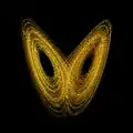
| ρ = 15, σ = 10, β = 8/3 (Enlarge) | ρ = 28, σ = 10, β = 8/3 (Enlarge) |
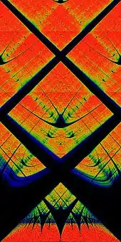
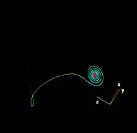
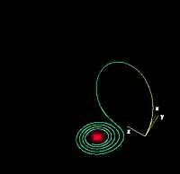
| For small values of ρ, the system is stable and evolves to one of two fixed point attractors. When ρ is larger than 24.74, the fixed points become repulsors and the trajectory is repelled by them in a very complex way. | |
| Sensitive dependence on the initial condition | ||
|---|---|---|
| Time t = 1 (Enlarge) | Time t = 2 (Enlarge) | Time t = 3 (Enlarge) |
 |
 |
 |
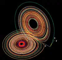
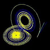
| These figures — made using ρ = 28, σ = 10 and β = 8/3 — show three time segments of the 3-D evolution of two trajectories (one in blue, the other in yellow) in the Lorenz attractor starting at two initial points that differ only by 10−5 in the x-coordinate. Initially, the two trajectories seem coincident (only the yellow one can be seen, as it is drawn over the blue one) but, after some time, the divergence is obvious. | ||
Connection to Tent Map
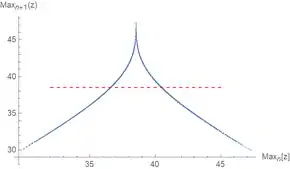
In Figure 4 of his paper,[1] Lorenz created a Poincaré plot by plotting the relative maximum value in the z direction achieved by the system, against the previous relative maximum in the z direction. The resulting plot has a shape very similar to the tent map. Lorenz also found that when the maximum z value is above a certain cut-off, the system will switch to the next lobe. Combining this with the chaos known to be exhibited by the tent map, he showed that the system switches between the two lobes chaotically.
Simulations
MATLAB simulation
% Solve over time interval [0,100] with initial conditions [1,1,1]
% ''f'' is set of differential equations
% ''a'' is array containing x, y, and z variables
% ''t'' is time variable

sigma = 10;
beta = 8/3;
rho = 28;
f = @(t,a) [-sigma*a(1) + sigma*a(2); rho*a(1) - a(2) - a(1)*a(3); -beta*a(3) + a(1)*a(2)];
[t,a] = ode45(f,[0 100],[1 1 1]);     % Runge-Kutta 4th/5th order ODE solver
plot3(a(:,1),a(:,2),a(:,3))
Mathematica simulation
Standard way:
tend = 50;
eq = {x'[t] == σ (y[t] - x[t]),
      y'[t] == x[t] (ρ - z[t]) - y[t],
      z'[t] == x[t] y[t] - β z[t]};
init = {x[0] == 10, y[0] == 10, z[0] == 10};
pars = {σ->10, ρ->28, β->8/3};
{xs, ys, zs} =
  NDSolveValue[{eq /. pars, init}, {x, y, z}, {t, 0, tend}];
ParametricPlot3D[{xs[t], ys[t], zs[t]}, {t, 0, tend}]
Less verbose:
lorenz = NonlinearStateSpaceModel[{{σ (y - x), x (ρ - z) - y, x y - β z}, {}}, {x, y, z}, {σ, ρ, β}];
soln[t_] = StateResponse[{lorenz, {10, 10, 10}}, {10, 28, 8/3}, {t, 0, 50}];
ParametricPlot3D[soln[t], {t, 0, 50}]
Dynamically interactive solution:
eqs = {
  x'[t] == σ (y[t] - x[t]), y'[t] == x[t] (ρ - z[t]) - y[t], z'[t] == x[t] y[t] - β z[t],
  x[0] == 10, y[0] == 10, z[0] == 10
};
tmax = 50;
sol = ParametricNDSolveValue[eqs, Function[t, {x[t], y[t], z[t]}], {t, 0, tmax}, {σ, ρ, β}];
Manipulate[
  fun = sol[σ, ρ, β];
  plot = ParametricPlot3D[fun[t], {t, 0, tmax}, PlotRange -> All, PerformanceGoal -> "Quality"];
  Animate[
    Show[plot, Graphics3D[{PointSize[0.05], Red, Point[fun[t]]}]],
    {t, 0, tmax}, AnimationRunning -> True, AnimationRate -> 1
  ],
  {{σ, 10}, 0, 100}, {{ρ, 28}, 0, 100}, {{β, 8/3}, 0, 100},
  TrackedSymbols :> {σ, ρ, β}
]
Python simulation
import numpy as np
import matplotlib.pyplot as plt
from scipy.integrate import odeint
from mpl_toolkits.mplot3d import Axes3D

rho = 28.0
sigma = 10.0
beta = 8.0 / 3.0

def f(state, t):
    x, y, z = state  # Unpack the state vector
    return sigma * (y - x), x * (rho - z) - y, x * y - beta * z  # Derivatives

state0 = [1.0, 1.0, 1.0]
t = np.arange(0.0, 40.0, 0.01)

states = odeint(f, state0, t)

fig = plt.figure()
ax = fig.gca(projection="3d")
ax.plot(states[:, 0], states[:, 1], states[:, 2])
plt.draw()
plt.show()
Modelica simulation
model LorenzSystem

  parameter Real sigma = 10;
  parameter Real rho = 28;
  parameter Real beta = 8/3;

  parameter Real x_start = 1 "Initial x-coordinate";
  parameter Real y_start = 1 "Initial y-coordinate";
  parameter Real z_start = 1 "Initial z-coordinate";

  Real x "x-coordinate";
  Real y "y-coordinate";
  Real z "z-coordinate";

initial equation
  x = x_start;
  y = y_start;
  z = z_start;

equation

  der(x) = sigma*(y-x);
  der(y) = rho*x - y - x*z;
  der(z) = x*y - beta*z;

end LorenzSystem;
Julia simulation
using DifferentialEquations, ParameterizedFunctions, Plots

lorenz = @ode_def begin                  # define the system
 dx = σ * (y - x)
 dy = x * (ρ - z) - y
 dz = x * y - β*z
end σ ρ β

u₀ = [1.0,0.0,0.0]                       # initial conditions
tspan = (0.0,100.0)                      # timespan
p = [10.0,28.0,8/3]                      # parameters
prob = ODEProblem(lorenz, u₀, tspan, p)  # define the problem
sol = solve(prob)                        # solve it
plot(sol, vars = (1, 2, 3))              # plot solution in phase space - variables ordered with 1 based indexing
Maxima simulation
load(dynamics)$
load(draw)$

/* System parameters */
a: 10; b: 8/3; r: 28;

lorenzSystem: [a*(y-x), -x*z+r*x-y, x*y-b*z];
dependentVariables: [x, y, z]$
initialValues: [1, 1, 1]$
timeRange: [t, 0, 50, 0.01]$

/* solution via 4th order Runge-Kutta method */
systemSolution: rk(lorenzSystem, dependentVariables, initialValues, timeRange)$
solutionPoints: map(lambda([x], rest(x)), systemSolution)$

draw3d(point_type=none, points_joined=true, color=blue,
       xlabel="x(t)", ylabel="y(t)", zlabel="z(t)",
       points(solutionPoints));
Derivation of the Lorenz equations as a model for atmospheric convection
The Lorenz equations are derived from the Oberbeck–Boussinesq approximation to the equations describing fluid circulation in a shallow layer of fluid, heated uniformly from below and cooled uniformly from above.[1] This fluid circulation is known as Rayleigh–Bénard convection. The fluid is assumed to circulate in two dimensions (vertical and horizontal) with periodic rectangular boundary conditions.
The partial differential equations modeling the system's stream function and temperature are subjected to a spectral Galerkin approximation: the hydrodynamic fields are expanded in Fourier series, which are then severely truncated to a single term for the stream function and two terms for the temperature. This reduces the model equations to a set of three coupled, nonlinear ordinary differential equations. A detailed derivation may be found, for example, in nonlinear dynamics texts.[21] The Lorenz system is a reduced version of a larger system studied earlier by Barry Saltzman.[22]
Resolution of Smale's 14th problem
Smale's 14th problem says 'Do the properties of the Lorenz attractor exhibit that of a strange attractor?', it was answered affirmatively by Warwick Tucker in 2002.[20] To prove this result, Tucker used rigorous numerics methods like interval arithmetic and normal forms. First, Tucker defined a cross section that is cut transversely by the flow trajectories. From this, one can define the first-return map , which assigns to each the point where the trajectory of first intersects .


Then the proof is split in three main points that are proved and imply the existence of a strange attractor.[23] The three points are:
- There exists a region invariant under the first-return map, meaning
- The return map admits a forward invariant cone field
- Vectors inside this invariant cone field are uniformly expanded by the derivative of the return map.


To prove the first point, we notice that the cross section is cut by two arcs formed by (see [23]). Tucker covers the location of these two arcs by small rectangles , the union of these rectangles gives . Now, the goal is to prove that for all points in , the flow will bring back the points in , in . To do that, we take a plan below at a distance small, then by taking the center of and using Euler integration method, one can estimate where the flow will bring in which gives us a new point . Then, one can estimate where the points in will be mapped in using Taylor expansion, this gives us a new rectangle centered on . Thus we know that all points in will be mapped in . The goal is to do this method recursively until the flow comes back to and we obtain a rectangle in such that we know that . The problem is that our estimation may become imprecise after several iterations, thus what Tucker does is to split into smaller rectangles and then apply the process recursively. Another problem is that as we are applying this algorithm, the flow becomes more 'horizontal' (see [23]), leading to a dramatic increase in imprecision. To prevent this, the algorithm changes the orientation of the cross sections, becoming either horizontal or vertical.


Contributions
Lorenz acknowledges the contributions from Ellen Fetter in his paper, who is responsible for the numerical simulations and figures.[1] Also, Margaret Hamilton helped in the initial, numerical computations leading up to the findings of the Lorenz model.[24]
Gallery
 A solution in the Lorenz attractor plotted at high resolution in the x-z plane.
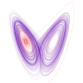 A solution in the Lorenz attractor rendered as an SVG.
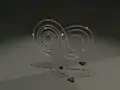 A solution in the Lorenz attractor rendered as a metal wire to show direction and 3D structure.
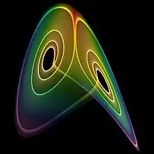 A visualization of the Lorenz attractor near an intermittent cycle.
 Two streamlines in a Lorenz system, from rho=0 to rho=28 (sigma=10, beta=8/3)
.gif) Animation of a Lorenz System with rho- dependence
Animation of a Lorenz System with rho- dependence
See also
- Eden's conjecture on the Lyapunov dimension
- Lorenz 96 model
- List of chaotic maps
- Takens' theorem
Notes
- Lorenz (1963)
- Sparrow (1982)
- Haken (1975)
- Knobloch (1981)
- Gorman, Widmann & Robbins (1986)
- Hemati (1994)
- Cuomo & Oppenheim (1993)
- Poland (1993)
- Tzenov (2014)
- Kolář & Gumbs (1992)
- Mishra & Sanghi (2006)
- Hirsch, Smale & Devaney (2003), pp. 303–305
- Hirsch, Smale & Devaney (2003), pp. 306+307
- Hirsch, Smale & Devaney (2003), pp. 307+308
- Kuznetsov, N.V.; Mokaev, T.N.; Kuznetsova, O.A.; Kudryashova, E.V. (2020). "The Lorenz system: hidden boundary of practical stability and the Lyapunov dimension". Nonlinear Dynamics. doi:10.1007/s11071-020-05856-4.
- Grassberger & Procaccia (1983)
- Leonov et al. (2016)
- Kuznetsov, Nikolay; Reitmann, Volker (2020). Attractor Dimension Estimates for Dynamical Systems: Theory and Computation. Cham: Springer.
- Guckenheimer, John; Williams, R. F. (1979-12-01). "Structural stability of Lorenz attractors". Publications Mathématiques de l'Institut des Hautes Études Scientifiques. 50 (1): 59–72. doi:10.1007/BF02684769. ISSN 0073-8301.
- Tucker (2002)
- Hilborn (2000), Appendix C; Bergé, Pomeau & Vidal (1984), Appendix D
- Saltzman (1962)
- Viana (2000)
- Lorenz (1960)
References
- Bergé, Pierre; Pomeau, Yves; Vidal, Christian (1984). Order within Chaos: Towards a Deterministic Approach to Turbulence. New York: John Wiley & Sons. ISBN 978-0-471-84967-4.
- Cuomo, Kevin M.; Oppenheim, Alan V. (1993). "Circuit implementation of synchronized chaos with applications to communications". Physical Review Letters. 71 (1): 65–68. Bibcode:1993PhRvL..71...65C. doi:10.1103/PhysRevLett.71.65. ISSN 0031-9007. PMID 10054374.
- Gorman, M.; Widmann, P.J.; Robbins, K.A. (1986). "Nonlinear dynamics of a convection loop: A quantitative comparison of experiment with theory". Physica D. 19 (2): 255–267. Bibcode:1986PhyD...19..255G. doi:10.1016/0167-2789(86)90022-9.
- Grassberger, P.; Procaccia, I. (1983). "Measuring the strangeness of strange attractors". Physica D. 9 (1–2): 189–208. Bibcode:1983PhyD....9..189G. doi:10.1016/0167-2789(83)90298-1.
- Haken, H. (1975). "Analogy between higher instabilities in fluids and lasers". Physics Letters A. 53 (1): 77–78. Bibcode:1975PhLA...53...77H. doi:10.1016/0375-9601(75)90353-9.
- Hemati, N. (1994). "Strange attractors in brushless DC motors". IEEE Transactions on Circuits and Systems I: Fundamental Theory and Applications. 41 (1): 40–45. doi:10.1109/81.260218. ISSN 1057-7122.
- Hilborn, Robert C. (2000). Chaos and Nonlinear Dynamics: An Introduction for Scientists and Engineers (second ed.). Oxford University Press. ISBN 978-0-19-850723-9.
- Hirsch, Morris W.; Smale, Stephen; Devaney, Robert (2003). Differential Equations, Dynamical Systems, & An Introduction to Chaos (Second ed.). Boston, MA: Academic Press. ISBN 978-0-12-349703-1.
- Knobloch, Edgar (1981). "Chaos in the segmented disc dynamo". Physics Letters A. 82 (9): 439–440. Bibcode:1981PhLA...82..439K. doi:10.1016/0375-9601(81)90274-7.
- Kolář, Miroslav; Gumbs, Godfrey (1992). "Theory for the experimental observation of chaos in a rotating waterwheel". Physical Review A. 45 (2): 626–637. doi:10.1103/PhysRevA.45.626. PMID 9907027.
- Leonov, G.A.; Kuznetsov, N.V.; Korzhemanova, N.A.; Kusakin, D.V. (2016). "Lyapunov dimension formula for the global attractor of the Lorenz system". Communications in Nonlinear Science and Numerical Simulation. 41: 84–103. arXiv:1508.07498. Bibcode:2016CNSNS..41...84L. doi:10.1016/j.cnsns.2016.04.032.
- Lorenz, Edward Norton (1963). "Deterministic nonperiodic flow". Journal of the Atmospheric Sciences. 20 (2): 130–141. Bibcode:1963JAtS...20..130L. doi:10.1175/1520-0469(1963)020<0130:DNF>2.0.CO;2.
- Mishra, Aashwin; Sanghi, Sanjeev (2006). "A study of the asymmetric Malkus waterwheel: The biased Lorenz equations". Chaos: An Interdisciplinary Journal of Nonlinear Science. 16 (1): 013114. Bibcode:2006Chaos..16a3114M. doi:10.1063/1.2154792. PMID 16599745.
- Pchelintsev, A.N. (2014). "Numerical and Physical Modeling of the Dynamics of the Lorenz System". Numerical Analysis and Applications. 7 (2): 159–167. doi:10.1134/S1995423914020098.
- Poland, Douglas (1993). "Cooperative catalysis and chemical chaos: a chemical model for the Lorenz equations". Physica D. 65 (1): 86–99. Bibcode:1993PhyD...65...86P. doi:10.1016/0167-2789(93)90006-M.
- Saltzman, Barry (1962). "Finite Amplitude Free Convection as an Initial Value Problem—I". Journal of the Atmospheric Sciences. 19 (4): 329–341. Bibcode:1962JAtS...19..329S. doi:10.1175/1520-0469(1962)019<0329:FAFCAA>2.0.CO;2.
- Sparrow, Colin (1982). The Lorenz Equations: Bifurcations, Chaos, and Strange Attractors. Springer.
- Tucker, Warwick (2002). "A Rigorous ODE Solver and Smale's 14th Problem" (PDF). Foundations of Computational Mathematics. 2 (1): 53–117. CiteSeerX 10.1.1.545.3996. doi:10.1007/s002080010018.
- Tzenov, Stephan (2014). "Strange Attractors Characterizing the Osmotic Instability". arXiv:1406.0979v1 [physics.flu-dyn].
- Viana, Marcelo (2000). "What's new on Lorenz strange attractors?". The Mathematical Intelligencer. 22 (3): 6–19. doi:10.1007/BF03025276.
- Lorenz, Edward N. (1960). "The statistical prediction of solutions of dynamic equations" (PDF). Symposium on Numerical Weather Prediction in Tokyo.
Further reading
- G.A. Leonov & N.V. Kuznetsov (2015). "On differences and similarities in the analysis of Lorenz, Chen, and Lu systems" (PDF). Applied Mathematics and Computation. 256: 334–343. doi:10.1016/j.amc.2014.12.132.
External links
| Wikimedia Commons has media related to Lorenz attractors. |
- "Lorenz attractor", Encyclopedia of Mathematics, EMS Press, 2001 [1994]
- Weisstein, Eric W. "Lorenz attractor". MathWorld.
- Lorenz attractor by Rob Morris, Wolfram Demonstrations Project.
- Lorenz equation on planetmath.org
- Synchronized Chaos and Private Communications, with Kevin Cuomo. The implementation of Lorenz attractor in an electronic circuit.
- Lorenz attractor interactive animation (you need the Adobe Shockwave plugin)
- 3D Attractors: Mac program to visualize and explore the Lorenz attractor in 3 dimensions
- Lorenz Attractor implemented in analog electronic
- Lorenz Attractor interactive animation (implemented in Ada with GTK+. Sources & executable)
- Web based Lorenz Attractor (implemented in JavaScript/HTML/CSS)
- Interactive web based Lorenz Attractor made with Iodide