Price equation

Example for a trait under positive selection

The Price equation shows that a change in the average amount ${\displaystyle z}$ of a trait in a population from one generation to the next (${\displaystyle \Delta z}$) is determined by the covariance between the amounts ${\displaystyle z_{i}}$ of the trait for subpopulation ${\displaystyle i}$ and the fitnesses ${\displaystyle w_{i}}$ of the subpopulations, together with the expected change in the amount of the trait value due to fitness, namely ${\displaystyle \mathrm {E} (w_{i}\Delta z_{i})}$:

${\displaystyle \Delta {z}={\frac {1}{w}}\operatorname {cov} (w_{i},z_{i})+{\frac {1}{w}}\operatorname {E} (w_{i}\,\Delta z_{i}).}$

Here ${\displaystyle w}$ is the average fitness over the population, and ${\displaystyle \operatorname {E} }$ and ${\displaystyle \operatorname {cov} }$ represent the population mean and covariance respectively. 'Fitness' ${\displaystyle w}$ is the ratio of the average number of offspring for the whole population per the number of adult individuals in the population, and ${\displaystyle w_{i}}$ is that same ratio only for subpopulation ${\displaystyle i}$.

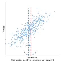
The covariance term captures the effects of natural selection; if the covariance between fitness (${\displaystyle w_{i}}$) and the trait value (${\displaystyle z_{i}}$) is positive then the trait value is predicted to increase on average over population ${\displaystyle i}$. If the covariance is negative then the trait is deleterious and is predicted to decrease in frequency.

The second term, ${\displaystyle \mathrm {E} (w_{i}\Delta z_{i})}$, represents factors other than direct selection that can affect trait evolution. This term can encompass genetic drift, mutation bias, or meiotic drive. Additionally, this term can encompass the effects of multi-level selection or group selection.

Price (1972) referred to this as the "environment change" term, and denoted both terms using partial derivative notation (∂_NS and ∂_EC). This concept of environment includes interspecies and ecological effects. Price describes this as follows:

Fisher adopted the somewhat unusual point of view of regarding dominance and epistasis as being environment effects. For example, he writes (1941): ‘A change in the proportion of any pair of genes itself constitutes a change in the environment in which individuals of the species find themselves.’ Hence he regarded the natural selection effect on M as being limited to the additive or linear effects of changes in gene frequencies, while everything else – dominance, epistasis, population pressure, climate, and interactions with other species – he regarded as a matter of the environment.

— G.R. Price (1972), Fisher's fundamental theorem made clear[2]

Suppose there is a population of ${\displaystyle n}$ individuals over which the amount of a particular characteristic varies. Those ${\displaystyle n}$ individuals can be grouped by the amount of the characteristic that each displays. There can be as few as just one group of all ${\displaystyle n}$ individuals (consisting of a single shared value of the characteristic) and as many as ${\displaystyle n}$ groups of one individual each (consisting of ${\displaystyle n}$ distinct values of the characteristic). Index each group with ${\displaystyle i}$ so that the number of members in the group is ${\displaystyle n_{i}}$ and the value of the characteristic shared among all members of the group is ${\displaystyle z_{i}}$. Now assume that having ${\displaystyle z_{i}}$ of the characteristic is associated with having a fitness ${\displaystyle w_{i}}$ where the product ${\displaystyle w_{i}n_{i}}$ represents the number of offspring in the next generation. Denote this number of offspring from group ${\displaystyle i}$ by ${\displaystyle n_{i}'}$ so that ${\displaystyle w_{i}=n_{i}'/n_{i}}$. Let ${\displaystyle z_{i}'}$ be the average amount of the characteristic displayed by the offspring from group ${\displaystyle i}$. Denote the amount of change in characteristic in group ${\displaystyle i}$ by ${\displaystyle \Delta z_{i}}$ defined by

${\displaystyle \Delta {z_{i}}\;{\stackrel {\mathrm {def} }{=}}\;z_{i}'-z_{i}}$

Now take ${\displaystyle z}$ to be the average characteristic value in this population and ${\displaystyle z'}$ to be the average characteristic value in the next generation. Define the change in average characteristic by ${\displaystyle \Delta {z}}$. That is,

${\displaystyle \Delta {z}\;{\stackrel {\mathrm {def} }{=}}\;z'-z}$

Note that this is not the average value of ${\displaystyle \Delta {z_{i}}}$ (as it is possible that ${\displaystyle n_{i}\neq n'_{i}}$). Also take ${\displaystyle w}$ to be the average fitness of this population. The Price equation states:

${\displaystyle w\,\Delta {z}=\operatorname {cov} (w_{i},z_{i})+\operatorname {E} (w_{i}\,\Delta z_{i})}$

where the functions ${\displaystyle \operatorname {E} }$ and ${\displaystyle \operatorname {cov} }$ are respectively defined in Equations (1) and (2) below and are equivalent to the traditional definitions of sample mean and covariance; however, they are not meant to be statistical estimates of characteristics of a population. In particular, the Price equation is a deterministic difference equation that models the trajectory of the actual mean value of a characteristic along the flow of an actual population of individuals. Assuming that the mean fitness ${\displaystyle w}$ is not zero, it is often useful to write it as

${\displaystyle \Delta {z}={\frac {1}{w}}\operatorname {cov} (w_{i},z_{i})+{\frac {1}{w}}\operatorname {E} (w_{i}\,\Delta z_{i})}$

In the specific case that characteristic ${\displaystyle z_{i}=w_{i}}$ (i.e., fitness itself is the characteristic of interest), then Price's equation reformulates Fisher's fundamental theorem of natural selection.

To prove the Price equation, the following definitions are needed. If ${\displaystyle n_{i}}$ is the number of occurrences of a pair of real numbers ${\displaystyle x_{i}}$ and ${\displaystyle y_{i}}$, then:

• The mean of the ${\displaystyle x_{i}}$ values is:

${\displaystyle \operatorname {E} (x_{i})\;{\stackrel {\mathrm {def} }{=}}\;{\frac {1}{\sum _{i}n_{i}}}\sum _{i}x_{i}n_{i}}$

${\displaystyle (1)}$

• The covariance between the ${\displaystyle x_{i}}$ and ${\displaystyle y_{i}}$ values is:

${\displaystyle \operatorname {cov} (x_{i},y_{i})\;{\stackrel {\mathrm {def} }{=}}\;{\frac {1}{\sum _{i}n_{i}}}\sum _{i}n_{i}[x_{i}-\operatorname {E} (x_{i})][y_{i}-\operatorname {E} (y_{i})]=\operatorname {E} (x_{i}y_{i})-\operatorname {E} (x_{i})\operatorname {E} (y_{i})}$

${\displaystyle (2)}$

The notation ${\displaystyle \langle x_{i}\rangle =\operatorname {E} (x_{i})}$ will also be used when convenient.

Suppose there is a population of organisms all of which have a genetic characteristic described by some real number. For example, high values of the number represent an increased visual acuity over some other organism with a lower value of the characteristic. Groups can be defined in the population which are characterized by having the same value of the characteristic. Let subscript ${\displaystyle i}$ identify the group with characteristic ${\displaystyle z_{i}}$ and let ${\displaystyle n_{i}}$ be the number of organisms in that group. The total number of organisms is then ${\displaystyle n}$ where:

${\displaystyle n=\sum _{i}n_{i}}$

The average value of the characteristic ${\displaystyle z}$ is defined as:

${\displaystyle z\;{\stackrel {\mathrm {def} }{=}}\;\operatorname {E} (z_{i})={\frac {1}{n}}\sum _{i}z_{i}n_{i}}$

${\displaystyle (3)}$

Now suppose that the population reproduces and the number of individuals in group ${\displaystyle i}$ in the next generation is represented by ${\displaystyle n'_{i}}$. The so-called fitness ${\displaystyle w_{i}}$ of group ${\displaystyle i}$ is defined to be the ratio of the number of its individuals in the next generation to the number of its individuals in the previous generation. That is,

${\displaystyle w_{i}={\frac {n_{i}'}{n_{i}}}}$

${\displaystyle (4)\,}$

Thus, saying that a group has "higher fitness" is equivalent to saying that its members produce more offspring per individual in the next generation. Similarly, ${\displaystyle n'}$ represents the total number of individuals across all groups, which can be expressed as:

${\displaystyle n'=\sum _{i}n'_{i}}$

Furthermore, the average fitness of the population can be shown to be the growth rate of the population as a whole, as in:

${\displaystyle w\;{\stackrel {\mathrm {def} }{=}}\;\operatorname {E} (w_{i})={\frac {1}{n}}\sum _{i}w_{i}n_{i}={\frac {1}{n}}\sum _{i}{\frac {n_{i}'}{n_{i}}}n_{i}={\frac {1}{n}}\sum _{i}n_{i}'={\frac {n'}{n}}}$

${\displaystyle (5)}$

Although the total population may grow, the proportion of individuals from a certain group may change. In particular, if one group has a higher fitness than another group, then the higher-fitness group will have a larger increase in representation in the next generation than the lower-fitness group. The average fitness represents how the population grows, and those groups with below-average fitness will tend to decline in proportion, while those groups with above-average fitness will tend to increase in proportion.

Along with the proportion of individuals in each group changing over time, the trait values within a single group may vary slightly from one generation to another (e.g., due to mutation). These two pressures together will cause the average value of the characteristic over the whole population to change over time. Assuming the value of ${\displaystyle z'_{i}}$ has changed by exactly the same amount for all members of the original group, in the new generation of the group, the average value ${\displaystyle z'}$ of the characteristic is:

${\displaystyle z'={\frac {1}{n'}}\sum _{i}z'_{i}n_{i}'}$

${\displaystyle (6)}$

where ${\displaystyle z'_{i}}$ are the (possibly new) values of the characteristic in group ${\displaystyle i}$. Equation (2) shows that:

${\displaystyle \operatorname {cov} (w_{i},z_{i})=\operatorname {E} (w_{i}z_{i})-wz}$

${\displaystyle (7)}$

Call the change in characteristic value from parent to child populations ${\displaystyle \Delta z_{i}}$ so that ${\displaystyle \Delta z_{i}=z'_{i}-z_{i}}$. As seen in Equation (1), the expected value operator ${\displaystyle \operatorname {E} }$ is linear, so

${\displaystyle \operatorname {E} (w_{i}\,\Delta z_{i})=\operatorname {E} (w_{i}z'_{i})-\operatorname {E} (w_{i}z_{i})}$

${\displaystyle (8)}$

Combining Equations (7) and (8) leads to

${\displaystyle \operatorname {cov} (w_{i},z_{i})+\operatorname {E} (w_{i}\,\Delta z_{i})=\left[\operatorname {E} (w_{i}z_{i})-wz\right]+\left[\operatorname {E} (w_{i}z'_{i})-\operatorname {E} (w_{i}z_{i})\right]=\operatorname {E} (w_{i}z'_{i})-wz}$

${\displaystyle (9)}$

Now, let's compute the first term in the equality above. From Equation (1), we know that:

${\displaystyle \operatorname {E} (w_{i}z'_{i})={\frac {1}{n}}\sum _{i}w_{i}z'_{i}n_{i}}$

Substituting the definition of fitness, ${\textstyle w_{i}={\frac {n'_{i}}{n_{i}}}}$ (Equation (4)), we get:

${\displaystyle \operatorname {E} (w_{i}z'_{i})={\frac {1}{n}}\sum _{i}{\frac {n'_{i}}{n_{i}}}z'_{i}n_{i}={\frac {1}{n}}\sum _{i}n'_{i}z'_{i}={\frac {n'}{n}}~{\frac {1}{n'}}\sum _{i}z'_{i}n'_{i}}$

${\displaystyle (10)}$

Next, substituting the definitions of average fitness (${\textstyle w={\frac {n'}{n}}}$) from Equation (5), and average child characteristics (${\textstyle z'}$) from Equation (6) gives the Price equation:

${\displaystyle \operatorname {cov} (w_{i},z_{i})+\operatorname {E} (w_{i}\,\Delta z_{i})=wz'-wz=w\,\Delta z\,}$

Derivation of the continuous-time Price equation

Consider a set of groups with ${\displaystyle i=1,...,n}$ that are characterized by a particular trait, denoted by ${\displaystyle x_{i}}$. The number ${\displaystyle n_{i}}$ of individuals belonging to group ${\displaystyle i}$ experiences exponential growth:

$${\displaystyle {dn_{i} \over {dt}}=f_{i}n_{i}}$$

where ${\displaystyle f_{i}}$ corresponds to the fitness of the group. We want to derive an equation describing the time-evolution of the expected value of the trait:

$${\displaystyle \mathbb {E} (x)=\sum _{i}p_{i}x_{i}\equiv \mu ,\quad p_{i}={n_{i} \over {\sum _{j}n_{j}}}}$$

Based on the chain rule, we may derive an ordinary differential equation:

$${\displaystyle {\begin{aligned}{d\mu \over {dt}}&=\sum _{i}{\partial \mu \over {\partial p_{i}}}{dp_{i} \over {dt}}+\sum _{i}{\partial \mu \over {\partial x_{i}}}{dx_{i} \over {dt}}\\&=\sum _{i}x_{i}{dp_{i} \over {dt}}+\sum _{i}p_{i}{dx_{i} \over {dt}}\\&=\sum _{i}x_{i}{dp_{i} \over {dt}}+\mathbb {E} \left({dx \over {dt}}\right)\end{aligned}}}$$

A further application of the chain rule for ${\displaystyle dp_{i}/dt}$ gives us:

$${\displaystyle {dp_{i} \over {dt}}=\sum _{j}{\partial p_{i} \over {\partial n_{j}}}{dn_{j} \over {dt}},\quad {\partial p_{i} \over {\partial n_{j}}}={\begin{cases}-p_{i}/N,\quad &i\neq j\\(1-p_{i})/N,\quad &i=j\end{cases}}}$$

Summing up the components gives us that:

$${\displaystyle {\begin{aligned}{dp_{i} \over {dt}}&=p_{i}\left(f_{i}-\sum _{j}p_{j}f_{j}\right)\\&=p_{i}\left[f_{i}-\mathbb {E} (f)\right]\end{aligned}}}$$

which is also known as the replicator equation. Now, note that:

$${\displaystyle {\begin{aligned}\sum _{i}x_{i}{dp_{i} \over {dt}}&=\sum _{i}p_{i}x_{i}\left[f_{i}-\mathbb {E} (f)\right]\\&=\mathbb {E} \left\{x_{i}\left[f_{i}-\mathbb {E} (f)\right]\right\}\\&={\text{Cov}}(x,f)\end{aligned}}}$$

Therefore, putting all of these components together, we arrive at the continuous-time Price equation:

$${\displaystyle {d \over {dt}}\mathbb {E} (x)=\underbrace {{\text{Cov}}(x,f)} _{\text{Selection effect}}+\underbrace {\mathbb {E} ({\dot {x}})} _{\text{Dynamic effect}}}$$

When the characteristic values ${\displaystyle z_{i}}$ do not change from the parent to the child generation, the second term in the Price equation becomes zero resulting in a simplified version of the Price equation:

${\displaystyle w\,\Delta z=\operatorname {cov} \left(w_{i},z_{i}\right)}$

which can be restated as:

${\displaystyle \Delta z=\operatorname {cov} \left(v_{i},z_{i}\right)}$

where ${\displaystyle v_{i}}$ is the fractional fitness: ${\displaystyle v_{i}=w_{i}/w}$.

This simple Price equation can be proven using the definition in Equation (2) above. It makes this fundamental statement about evolution: "If a certain inheritable characteristic is correlated with an increase in fractional fitness, the average value of that characteristic in the child population will be increased over that in the parent population."

The simple Price equation was based on the assumption that the characters ${\displaystyle z_{i}}$ do not change over one generation. If it is assumed that they do change, with ${\displaystyle z_{i}}$ being the value of the character in the child population, then the full Price equation must be used. A change in character can come about in a number of ways. The following two examples illustrate two such possibilities, each of which introduces new insight into the Price equation.

The use of the change in average characteristic (${\displaystyle z'-z}$) per generation as a measure of evolutionary progress is not always appropriate. There may be cases where the average remains unchanged (and the covariance between fitness and characteristic is zero) while evolution is nevertheless in progress.

A critical discussion of the use of the Price equation can be found in van Veelen (2005),[3] van Veelen et al. (2012),[4] and van Veelen (2020).[5] Frank (2012) discusses the criticism in van Veelen et al. (2012).[6]

Price's equation features in the plot and title of the 2008 thriller film WΔZ.

The Price equation also features in posters in the computer game BioShock 2, in which a consumer of a "Brain Boost" tonic is seen deriving the Price equation while simultaneously reading a book. The game is set in the 1950s, substantially before Price's work.

• Price equation examples

References

- Knudsen, Thorbjørn (2004). "General selection theory and economic evolution: The Price equation and the replicator/interactor distinction". Journal of Economic Methodology. 11 (2): 147–173. doi:10.1080/13501780410001694109. S2CID 154197796. Retrieved 2011-10-22.
- Price, G.R. (1972). "Fisher's "fundamental theorem" made clear". Annals of Human Genetics. 36 (2): 129–140. doi:10.1111/j.1469-1809.1972.tb00764.x. PMID 4656569. S2CID 20757537.
- van Veelen, M. (December 2005). "On the use of the Price equation". Journal of Theoretical Biology. 237 (4): 412–426. doi:10.1016/j.jtbi.2005.04.026. PMID 15953618.
- van Veelen, M.; García, J.; Sabelis, M.W.; Egas, M. (April 2012). "Group selection and inclusive fitness are not equivalent; the Price equation vs. models and statistics". Journal of Theoretical Biology. 299: 64–80. doi:10.1016/j.jtbi.2011.07.025. PMID 21839750.
- van Veelen, M. (March 2020). "The problem with the Price equation". Philosophical Transactions of the Royal Society B. 375 (1797): 1–13. doi:10.1098/rstb.2019.0355. PMC 7133513. PMID 32146887.
- Frank, S.A. (2012). "Natural Selection IV: The Price equation". Journal of Evolutionary Biology. 25 (6): 1002–1019. arXiv:1204.1515. doi:10.1111/j.1420-9101.2012.02498.x. PMC 3354028. PMID 22487312.
Further reading
- Frank, S.A. (1995). "George Price's contributions to Evolutionary Genetics" (PDF). Journal of Theoretical Biology. 175 (3): 373–388. CiteSeerX 10.1.1.136.7803. doi:10.1006/jtbi.1995.0148. PMID 7475081.
- Frank, S.A. (1997). "The Price equation, Fisher's fundamental theorem, kin selection, and causal analysis" (PDF). Evolution. 51 (6): 1712–1729. doi:10.2307/2410995. JSTOR 2410995. PMID 28565119.
- Gardner, A. (2008). "The Price equation" (PDF). Curr. Biol. 18 (5): R198–R202. doi:10.1016/j.cub.2008.01.005. PMID 18334191. S2CID 1169263. Archived from the original (PDF) on 2008-12-16.
- Grafen, A. (2000). "Developments of the Price equation and natural selection under uncertainty" (PDF). Proceedings of the Royal Society B. 267 (1449): 1223–1227. doi:10.1098/rspb.2000.1131. PMC 1690660. PMID 10902688.
- Harman, Oren (2010). The Price of Altruism: George Price and the search for the origins of kindness. Bodley Head. ISBN 978-1-84792-062-1.
- Langdon, W.B. (1998). "8.1 Evolution of GP populations: Price's selection and covariance theorem". Genetic Programming and Data Structures. pp. 167–208.
- Price, G.R. (1970). "Selection and covariance" (PDF). Nature. 227 (5257): 520–521. Bibcode:1970Natur.227..520P. doi:10.1038/227520a0. PMID 5428476. S2CID 4264723.
- Price, G.R. (1972). "Extension of covariance selection mathematics". Annals of Human Genetics. 35 (4): 485–490. doi:10.1111/j.1469-1809.1957.tb01874.x. PMID 5073694. S2CID 37828617.
- van Veelen, Matthijs; García, Julián; Sabelis, Maurice W. & Egas, Martijn (2010). "Call for a return to rigour in models". Correspondence. Nature. 467 (7316): 661. Bibcode:2010Natur.467..661V. doi:10.1038/467661d. PMID 20930826.
- Day, T. (2006). "Insights from Price's equation into evolutionary epidemiology". Insights from Price's equation into evolutionnary epidemiology. DIMACS Series in Discrete Mathematics and Theoretical Computer Science. 71. pp. 23–43. doi:10.1090/dimacs/071/02. ISBN 9780821837535.
- "How to quit the Price equation: An online self-help tutorial".
- "The Good Show". Radiolab. Season 9. Episode 1. New York. 14 December 2011. WNYC.
- Markovitch; Witkowski; Virgo (2018). "Chemical heredity as group selection at the molecular level". arXiv:1802.08024 [q-bio.PE].