Spline interpolation

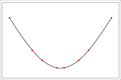
Originally, spline was a term for elastic rulers that were bent to pass through a number of predefined points, or knots. These were used to make technical drawings for shipbuilding and construction by hand, as illustrated by Figure 1.

Figure 1: Interpolation with cubic splines between eight points. Hand-drawn technical drawings were made for shipbuilding etc. using flexible rulers that were bent to follow pre-defined points

We wish to model similar kinds of curves using a set of mathematical equations, with one polynomial ${\displaystyle y=q_{i}(x)}$ for each pair of knots, ${\displaystyle (x_{i-1},y_{i-1})}$ and ${\displaystyle (x_{i},y_{i})}$, where ${\displaystyle i=1,2,\cdots ,n}$. So there will be ${\displaystyle n}$ polynomials, and ${\displaystyle n+1}$ knots: The first polynomial starts at ${\displaystyle (x_{0},y_{0})}$, and the last polynomial ends at ${\displaystyle (x_{n},y_{n})}$.

The curvature of any curve ${\displaystyle y=f(x)}$ is defined as:

${\displaystyle \kappa ={\frac {y''}{(1+y'^{2})^{3/2}}}}$

To make the spline take a shape that minimizes the bending (under the constraint of passing through all knots), we will define both ${\displaystyle y'}$ and ${\displaystyle y''}$ to be continuous everywhere, including at the knots. Thus the first and second derivatives of each successive polynomial must have identical values at the knots, which is to say that

${\displaystyle {\begin{cases}q'_{i}(x_{i})=q'_{i+1}(x_{i})\\q''_{i}(x_{i})=q''_{i+1}(x_{i})\end{cases}}\qquad 1\leq i\leq n-1}$

This can only be achieved if polynomials of degree 3 or higher — cubic polynomials or higher — are used. The classical approach is to use polynomials of exactly degree 3 — cubic splines.

We wish to find each polynomial ${\displaystyle q_{i}(x)}$ given the points ${\displaystyle (x_{0},y_{0})}$ through ${\displaystyle (x_{n},y_{n})}$. To do this, we will consider just a single piece of the curve, ${\displaystyle q(x)}$, which will interpolate from ${\displaystyle (x_{1},y_{1})}$ to ${\displaystyle (x_{2},y_{2})}$. This piece will have slopes ${\displaystyle k_{1}}$ and ${\displaystyle k_{2}}$ at its endpoints. Or, more precisely:

${\displaystyle q(x_{1})=y_{1}}$

${\displaystyle q(x_{2})=y_{2}}$

${\displaystyle q'(x_{1})=k_{1}}$

${\displaystyle q'(x_{2})=k_{2}}$

The full equation ${\displaystyle q(x)}$ can be written in the symmetrical form

${\displaystyle q(x)={\big (}1-t(x){\big )}\,y_{1}+t(x)\,y_{2}+t(x){\big (}1-t(x){\big )}{\Big (}{\big (}1-t(x){\big )}\,a+t(x)\,b{\Big )}}$

(1)

where

${\displaystyle t(x)={\frac {x-x_{1}}{x_{2}-x_{1}}},}$

(2)

${\displaystyle a=k_{1}(x_{2}-x_{1})-(y_{2}-y_{1}),}$

(3)

${\displaystyle b=-k_{2}(x_{2}-x_{1})+(y_{2}-y_{1}).}$

(4)

But what are ${\displaystyle k_{1}}$ and ${\displaystyle k_{2}}$? To derive these critical values, we must consider that

${\displaystyle q'={\frac {dq}{dx}}={\frac {dq}{dt}}{\frac {dt}{dx}}={\frac {dq}{dt}}{\frac {1}{x_{2}-x_{1}}}}$

It then follows that

${\displaystyle q'={\frac {y_{2}-y_{1}}{x_{2}-x_{1}}}+(1-2t){\frac {a(1-t)+bt}{x_{2}-x_{1}}}+t(1-t){\frac {b-a}{x_{2}-x_{1}}},}$

(5)

${\displaystyle q''=2{\frac {b-2a+(a-b)3t}{{(x_{2}-x_{1})}^{2}}}.}$

(6)

Setting t = 0 and t = 1 respectively in equations (5) and (6) one gets from (2) that indeed first derivatives q′(x₁) = k₁ and q′(x₂) = k₂ and also second derivatives

${\displaystyle q''(x_{1})=2{\frac {b-2a}{{(x_{2}-x_{1})}^{2}}}}$

(7)

${\displaystyle q''(x_{2})=2{\frac {a-2b}{{(x_{2}-x_{1})}^{2}}}}$

(8)

If now (x_i, y_i), i = 0, 1, ..., n are n + 1 points and

${\displaystyle q_{i}=(1-t)\,y_{i-1}+t\,y_{i}+t(1-t){\big (}(1-t)\,a_{i}+t\,b_{i}{\big )}}$

(9)

where i = 1, 2, ..., n and ${\displaystyle t={\tfrac {x-x_{i-1}}{x_{i}-x_{i-1}}}}$ are n third degree polynomials interpolating y in the interval x_i−1 ≤ x ≤ x_i for i = 1, ..., n such that q′_i (x_i) = q′_i+1(x_i) for i = 1, ..., n−1 then the n polynomials together define a differentiable function in the interval x₀ ≤ x ≤ x_n and

${\displaystyle a_{i}=k_{i-1}(x_{i}-x_{i-1})-(y_{i}-y_{i-1})}$

(10)

${\displaystyle b_{i}=-k_{i}(x_{i}-x_{i-1})+(y_{i}-y_{i-1})}$

(11)

for i = 1, ..., n where

${\displaystyle k_{0}=q_{1}'(x_{0})}$

(12)

${\displaystyle k_{i}=q_{i}'(x_{i})=q_{i+1}'(x_{i})\qquad i=1,\dotsc ,n-1}$

(13)

${\displaystyle k_{n}=q_{n}'(x_{n})}$

(14)

If the sequence k₀, k₁, ..., k_n is such that, in addition, q′′_i(x_i) = q′′_i+1(x_i) holds for i = 1, ..., n-1, then the resulting function will even have a continuous second derivative.

From (7), (8), (10) and (11) follows that this is the case if and only if

${\displaystyle {\frac {k_{i-1}}{x_{i}-x_{i-1}}}+\left({\frac {1}{x_{i}-x_{i-1}}}+{\frac {1}{x_{i+1}-x_{i}}}\right)2k_{i}+{\frac {k_{i+1}}{x_{i+1}-x_{i}}}=3\left({\frac {y_{i}-y_{i-1}}{{(x_{i}-x_{i-1})}^{2}}}+{\frac {y_{i+1}-y_{i}}{{(x_{i+1}-x_{i})}^{2}}}\right)}$

(15)

for i = 1, ..., n-1. The relations (15) are n − 1 linear equations for the n + 1 values k₀, k₁, ..., k_n.

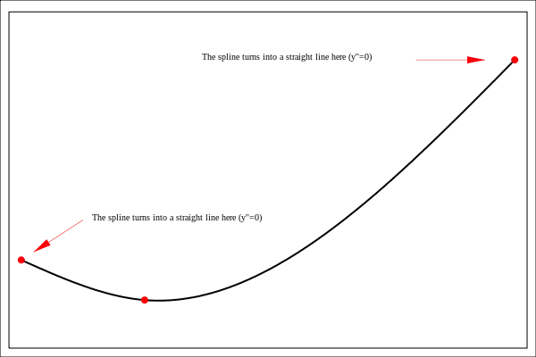
For the elastic rulers being the model for the spline interpolation one has that to the left of the left-most "knot" and to the right of the right-most "knot" the ruler can move freely and will therefore take the form of a straight line with q′′ = 0. As q′′ should be a continuous function of x one gets that for "Natural Splines" one in addition to the n − 1 linear equations (15) should have that

${\displaystyle q''_{1}(x_{0})=2{\frac {3(y_{1}-y_{0})-(k_{1}+2k_{0})(x_{1}-x_{0})}{{(x_{1}-x_{0})}^{2}}}=0,}$

${\displaystyle q''_{n}(x_{n})=-2{\frac {3(y_{n}-y_{n-1})-(2k_{n}+k_{n-1})(x_{n}-x_{n-1})}{{(x_{n}-x_{n-1})}^{2}}}=0,}$

i.e. that

${\displaystyle {\frac {2}{x_{1}-x_{0}}}k_{0}+{\frac {1}{x_{1}-x_{0}}}k_{1}=3{\frac {y_{1}-y_{0}}{(x_{1}-x_{0})^{2}}},}$

(16)

${\displaystyle {\frac {1}{x_{n}-x_{n-1}}}k_{n-1}+{\frac {2}{x_{n}-x_{n-1}}}k_{n}=3{\frac {y_{n}-y_{n-1}}{(x_{n}-x_{n-1})^{2}}}.}$

(17)

Eventually, (15) together with (16) and (17) constitute n + 1 linear equations that uniquely define the n + 1 parameters k₀, k₁, ..., k_n.

There exist other end conditions: "Clamped spline", that specifies the slope at the ends of the spline, and the popular "not-a-knot spline", that requires that the third derivative is also continuous at the x₁ and x_N−1 points. For the "not-a-knot" spline, the additional equations will read:

${\displaystyle q'''_{1}(x_{1})=q'''_{2}(x_{1})\Rightarrow {\frac {1}{\Delta x_{1}^{2}}}k_{0}+\left({\frac {1}{\Delta x_{1}^{2}}}-{\frac {1}{\Delta x_{2}^{2}}}\right)k_{1}-{\frac {1}{\Delta x_{2}^{2}}}k_{2}=2\left({\frac {\Delta y_{1}}{\Delta x_{1}^{3}}}-{\frac {\Delta y_{2}}{\Delta x_{2}^{3}}}\right)}$

${\displaystyle q'''_{n-1}(x_{n-1})=q'''_{n}(x_{n-1})\Rightarrow {\frac {1}{\Delta x_{n-1}^{2}}}k_{n-2}+\left({\frac {1}{\Delta x_{n-1}^{2}}}-{\frac {1}{\Delta x_{n}^{2}}}\right)k_{n-1}-{\frac {1}{\Delta x_{n}^{2}}}k_{n}=2\left({\frac {\Delta y_{n-1}}{\Delta x_{n-1}^{3}}}-{\frac {\Delta y_{n}}{\Delta x_{n}^{3}}}\right)}$

where ${\displaystyle \Delta x_{i}=x_{i}-x_{i-1},\Delta y_{i}=y_{i}-y_{i-1}}$.

Figure 2: Interpolation with cubic "natural" splines between three points.

In case of three points the values for ${\displaystyle k_{0},k_{1},k_{2}}$ are found by solving the tridiagonal linear equation system

${\displaystyle {\begin{bmatrix}a_{11}&a_{12}&0\\a_{21}&a_{22}&a_{23}\\0&a_{32}&a_{33}\\\end{bmatrix}}{\begin{bmatrix}k_{0}\\k_{1}\\k_{2}\\\end{bmatrix}}={\begin{bmatrix}b_{1}\\b_{2}\\b_{3}\\\end{bmatrix}}}$

with

${\displaystyle a_{11}={\frac {2}{x_{1}-x_{0}}}}$

${\displaystyle a_{12}={\frac {1}{x_{1}-x_{0}}}}$

${\displaystyle a_{21}={\frac {1}{x_{1}-x_{0}}}}$

${\displaystyle a_{22}=2\ \left({\frac {1}{x_{1}-x_{0}}}+{\frac {1}{x_{2}-x_{1}}}\right)}$

${\displaystyle a_{23}={\frac {1}{x_{2}-x_{1}}}}$

${\displaystyle a_{32}={\frac {1}{x_{2}-x_{1}}}}$

${\displaystyle a_{33}={\frac {2}{x_{2}-x_{1}}}}$

${\displaystyle b_{1}=3\ {\frac {y_{1}-y_{0}}{(x_{1}-x_{0})^{2}}}}$

${\displaystyle b_{2}=3\ \left({\frac {y_{1}-y_{0}}{{(x_{1}-x_{0})}^{2}}}+{\frac {y_{2}-y_{1}}{{(x_{2}-x_{1})}^{2}}}\right)}$

${\displaystyle b_{3}=3\ {\frac {y_{2}-y_{1}}{(x_{2}-x_{1})^{2}}}}$

For the three points

${\displaystyle (-1,0.5)\ ,\ (0,0)\ ,\ (3,3)}$,

one gets that

${\displaystyle k_{0}=-0.6875\ ,\ k_{1}=-0.1250\ ,\ k_{2}=1.5625}$

and from (10) and (11) that

${\displaystyle a_{1}=k_{0}(x_{1}-x_{0})-(y_{1}-y_{0})=-0.1875}$

${\displaystyle b_{1}=-k_{1}(x_{1}-x_{0})+(y_{1}-y_{0})=-0.3750}$

${\displaystyle a_{2}=k_{1}(x_{2}-x_{1})-(y_{2}-y_{1})=-3.3750}$

${\displaystyle b_{2}=-k_{2}(x_{2}-x_{1})+(y_{2}-y_{1})=-1.6875}$

In Figure 2, the spline function consisting of the two cubic polynomials ${\displaystyle q_{1}(x)}$ and ${\displaystyle q_{2}(x)}$ given by (9) is displayed.

• Cubic Hermite spline
• Centripetal Catmull–Rom spline
• Discrete spline interpolation
• Monotone cubic interpolation
• NURBS
• Multivariate interpolation
• Polynomial interpolation
• Smoothing spline
• Spline wavelet
• Thin plate spline
• Polyharmonic spline

TinySpline: Open source C-library for splines which implements cubic spline interpolation

SciPy Spline Interpolation: a Python package that implements interpolation

Cubic Interpolation: Open source C#-library for cubic spline interpolation

• Schoenberg, Isaac J. (1946). "Contributions to the Problem of Approximation of Equidistant Data by Analytic Functions: Part A.—On the Problem of Smoothing or Graduation. A First Class of Analytic Approximation Formulae". Quarterly of Applied Mathematics. 4 (2): 45–99. doi:10.1090/qam/15914.CS1 maint: ref=harv (link)
• Schoenberg, Isaac J. (1946). "Contributions to the Problem of Approximation of Equidistant Data by Analytic Functions: Part B.—On the Problem of Osculatory Interpolation. A Second Class of Analytic Approximation Formulae". Quarterly of Applied Mathematics. 4 (2): 112–141. doi:10.1090/qam/16705.CS1 maint: ref=harv (link)

• Cubic Spline Interpolation Online Calculation and Visualization Tool (with JavaScript source code)
• "Spline interpolation", Encyclopedia of Mathematics, EMS Press, 2001 [1994]
• Dynamic cubic splines with JSXGraph
• Lectures on the theory and practice of spline interpolation
• Paper which explains step by step how cubic spline interpolation is done, but only for equidistant knots.
• Numerical Recipes in C, Go to Chapter 3 Section 3-3
• A note on cubic splines
• Information about spline interpolation (including code in Fortran 77)

References

- Hall, Charles A.; Meyer, Weston W. (1976). "Optimal Error Bounds for Cubic Spline Interpolation". Journal of Approximation Theory. 16 (2): 105–122. doi:10.1016/0021-9045(76)90040-X.