Configuration model
In network science, the configuration model is a method for generating random networks from given degree sequence. It is widely used as a reference model for real-life social networks, because it allows the user to incorporate arbitrary degree distributions.
| Network science | ||||
|---|---|---|---|---|
| Network types | ||||
| Graphs | ||||
|
||||
| Models | ||||
|
||||
| ||||
|
||||
Rationale for the model
In the configuration model, the degree of each vertex is pre-defined, rather than having a probability distribution from which the given degree is chosen.[2] As opposed to the Erdős-Rényi model, the degree sequence of the configuration model is not restricted to have a Poisson-distribution, the model allows the user to give the network any desired degree distribution.
Algorithm
The following algorithm describes the generation of the model:
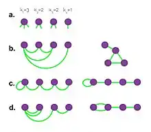
- Take a degree sequence, i. e. assign a degree to each vertex. The degrees of the vertices are represented as half-links or stubs. The sum of stubs must be even in order to be able to construct a graph (). The degree sequence can be drawn from a theoretical distribution or it can represent a real network (determined from the adjacency matrix of the network).
- Choose two stubs uniformly at random and connect them to form an edge. Choose another pair from the remaining stubs and connect them. Continue until you run out of stubs. The result is a network with the pre-defined degree sequence. The realization of the network changes with the order in which the stubs are chosen, they might include cycles (b), self-loops (c) or multi-links (d) (Figure 1) Yet, the expected number of self-loops and multi-links goes to zero in the N → ∞ limit.[1]


Self-loops, multi-edges and implications
The algorithm described above matches any stubs with the same probability. The uniform distribution of the matching is an important property in terms of calculating other features of the generated networks. The network generation process does not exclude the event of generating a self-loop or a multi-link. If we designed the process where self-loops and multi-edges are not allowed, the matching of the stubs would not follow a uniform distribution. However, the average number of self-loops and multi-edges is a constant for large networks, so the density of self-loops and multi-links goes to zero as [2] (see the cited book for details).

A further consequence of self-loops and multi-edges is that not all possible networks are generated with the same probability. In general, all possible realizations can be generated by permuting the stubs of all vertices in every possible way. The number of permutation of the stubs of node is , so the number of realizations of a degree sequence is . This would mean that each realization occurs with the same probability. However, self-loops and multi-edges can change the number of realizations, since permuting self-edges can result an unchanged realization. Given that the number of self-loops and multi-links vanishes as , the variation in probabilities of different realization will be small but present.[2]


Properties
Edge probability
A stub of node can be connected to other stubs (there are stubs altogether, and we have to exclude the one we are currently observing). The vertex has stubs to which node can be connected with the same probability (because of the uniform distribution). The probability of a stub of node being connected to one of these stubs is . Since node has stubs, the probability of being connected to is ( for sufficiently large ). The probability of self-edges cannot be described by this formula, but as the density of self-edges goes to zero as , it usually gives a good estimate.[2]


Given a configuration model with a degree distribution , the probability of a randomly chosen node having degree is . But if we took one of the vertices to which we can arrive following one of edges of i, the probability of having degree k is . (The probability of reaching a node with degree k is , and there are such nodes.) This fraction depends on as opposed to the degree of the typical node with . Thus, a neighbor of a typical node is expected to have higher degree than the typical node itself. This feature of the configuration model describes well the phenomenon of "my friends having more friends than I do".


Clustering coefficient
The global clustering coefficient (the average probability that the neighbors of a node are connected) is computed as follows:

,

where denotes the probabilistic distributions of vertices and having edges, respectively.


After transforming the equation above, we get approximately
, where is the number of vertices, and the size of the constant depends on .[2] Thus, the global clustering coefficient becomes small at large n limit.


Giant component
In the configuration model, a giant component (GC) exists if

where and are the first and second moments of the degree distribution. That means that, the critical threshold solely depends on quantities which are uniquely determined by the degree distribution .


Configuration model generates locally tree-like networks, meaning that any local neighborhood in such a network takes the form of a tree. More precisely, if you start at any node in the network and form the set of all nodes at distance or less from that starting node, the set will, with probability tending to 1 as n → ∞, take the form of a tree.[3] In tree-like structures, the number of second neighbors averaged over the whole network, , is:


Then, in general, the average number at distance can be written as:

Which implies that if the ratio of is larger than one, then the network can have a giant component. This is famous as the Molloy-Reed criterion.[4] The intuition behind this criterion is that if the giant component exists, then the average degree of a randomly chosen vertex in a connected component should be at least 2. Molloy-Reed criterion can also be expressed as: which implies that, although the size of the GC may depend on and , the number of nodes of degree 0 and 2 have no contribution in the existence of the giant component.[3]


Diameter
Configuration model can assume any degree distribution and shows the small-world effect, since to leading order the diameter of the configuration model is just .[5]

Components of finite size
As total number of vertices tends to infinity, the probability to find two giant components is vanishing. This means that in the sparse regime, the model consist of one giant component (if any) and multiple connected components of finite size. The sizes of the connected components are characterized by their size distribution - the probability that a randomly sampled vertex belongs to a connected component of size There is a correspondence between the degree distribution and the size distribution When total number of vertices tends to infinity, , the following relation takes place:[6]


where and denotes the -fold convolution power. Moreover, explicit asymptotes for are known when and is close to zero.[6] The analytical expressions for these asymptotes depend on finiteness of the moments of the degree distribution tail exponent (when features a heavy tail), and the sign of Molloy-Reed criterium. The following table summarises these relationships (the constants are provided in[6]).


| Moments of | Tail of | ||
|---|---|---|---|
| light tail | -1 or 1 | ||
| 0 | |||
| heavy tail, | -1 | ||
| 0 | |||
| 1 | |||
|
|
heavy tail, | -1 | |
| 0 | |||
| 1 | |||
| heavy tail, | -1 | ||
| 0 | |||
| 1 | |||
|
|
heavy tail, | 1 | |
| heavy tail, | 1 |


Modelling
Comparison to real-world networks
Three general properties of complex networks are heterogeneous degree distribution, short average path length and high clustering.[1][7][8] Having the opportunity to define any arbitrary degree sequence, the first condition can be satisfied by design, but as shown above, the global clustering coefficient is an inverse function of the network size, so for large configuration networks, clustering tends to be small. This feature of the baseline model contradicts the known properties of empirical networks, but extensions of the model can solve this issue (see [9]).
Application: modularity calculation
The configuration model is applied as benchmark in the calculation of network modularity. Modularity measures the degree of division of the network into modules. It is computed as follows:

in which the adjacency matrix of the network is compared to the probability of having an edge between node and (depending on their degrees) in the configuration model (see the page modularity for details).
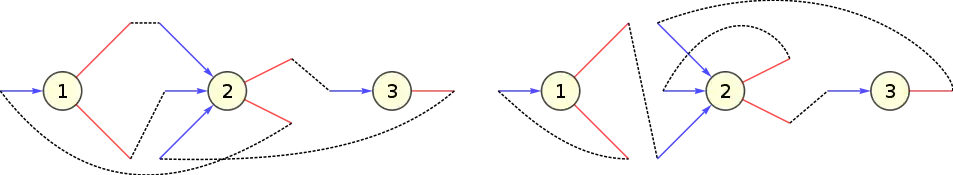
Directed configuration model
In the DCM (directed configuration model),[11] each node is given a number of half-edges called tails and heads. Then tails and heads are matched uniformly at random to form directed edges. The size of the giant component,[11][12] the typical distance,[13] and the diameter[14] of DCM have been studied mathematically. There also has been extensive research on random walks on DCM.[15][16][17] Some real-world complex networks have been modelled by DCM, such as neural networks,[18] finance[19] and social networks.[20]
References
- Network Science by Albert-László Barabási.
- Newman, Mark (2010-03-25). Networks: An Introduction - Oxford Scholarship. Oxford University Press. doi:10.1093/acprof:oso/9780199206650.001.0001. ISBN 9780191594175.
- Newman, Mark (2018-10-18). Networks. 1. Oxford University Press. doi:10.1093/oso/9780198805090.001.0001. ISBN 978-0-19-880509-0.
- Molloy, Michael; Reed, Bruce (1995-03-01). "A critical point for random graphs with a given degree sequence". Random Structures & Algorithms. 6 (2–3): 161–180. CiteSeerX 10.1.1.24.6195. doi:10.1002/rsa.3240060204. ISSN 1098-2418.
- Chung, Fan; Lu, Linyuan (2002-12-10). "The average distances in random graphs with given expected degrees". Proceedings of the National Academy of Sciences. 99 (25): 15879–15882. Bibcode:2002PNAS...9915879C. doi:10.1073/pnas.252631999. ISSN 0027-8424. PMC 138532. PMID 12466502.
- Kryven, I (2017). "General expression for the component size distribution in infinite configuration networks". Physical Review E. 95 (5): 052303. arXiv:1703.05413. Bibcode:2017PhRvE..95e2303K. doi:10.1103/PhysRevE.95.052303. hdl:11245.1/fa1b270b-61a5-4f20-b496-ddf446fdfe80. PMID 28618550. S2CID 8421307.
- Barabási, Albert-László; Albert, Réka (1999-10-15). "Emergence of Scaling in Random Networks". Science. 286 (5439): 509–512. arXiv:cond-mat/9910332. Bibcode:1999Sci...286..509B. doi:10.1126/science.286.5439.509. ISSN 0036-8075. PMID 10521342. S2CID 524106.
- Watts, Duncan J.; Strogatz, Steven H. (1998). "Collective dynamics of 'small-world' networks". Nature. 393 (6684): 440–442. Bibcode:1998Natur.393..440W. doi:10.1038/30918. ISSN 1476-4687. PMID 9623998. S2CID 4429113.
- Newman, M. E. J. (2009). "Random Graphs with Clustering". Physical Review Letters. 103 (5): 058701. arXiv:0903.4009. Bibcode:2009PhRvL.103e8701N. doi:10.1103/physrevlett.103.058701. PMID 19792540. S2CID 28214709.
- Newman, M. E. J. (2004). "Finding and evaluating community structure in networks". Physical Review E. 69 (2): 026113. arXiv:cond-mat/0308217. Bibcode:2004PhRvE..69b6113N. doi:10.1103/physreve.69.026113. PMID 14995526. S2CID 197314.
- COOPER, COLIN; FRIEZE, ALAN (May 2004). "The Size of the Largest Strongly Connected Component of a Random Digraph with a Given Degree Sequence". Combinatorics, Probability and Computing. 13 (3): 319–337. doi:10.1017/S096354830400611X. ISSN 1469-2163.
- Cai, Xing Shi; Perarnau, Guillem (10 April 2020). "The giant component of the directed configuration model revisited". arXiv:2004.04998 [math.PR].
- van der Hoorn, Pim; Olvera-Cravioto, Mariana (June 2018). "Typical distances in the directed configuration model". The Annals of Applied Probability. 28 (3): 1739–1792. arXiv:1511.04553. doi:10.1214/17-AAP1342. S2CID 13683470.
- Cai, Xing Shi; Perarnau, Guillem (10 March 2020). "The diameter of the directed configuration model". arXiv:2003.04965 [math.PR].
- Bordenave, Charles; Caputo, Pietro; Salez, Justin (1 April 2018). "Random walk on sparse random digraphs". Probability Theory and Related Fields. 170 (3): 933–960. arXiv:1508.06600. doi:10.1007/s00440-017-0796-7. ISSN 1432-2064. S2CID 55211047.
- Caputo, Pietro; Quattropani, Matteo (1 December 2020). "Stationary distribution and cover time of sparse directed configuration models". Probability Theory and Related Fields. 178 (3): 1011–1066. doi:10.1007/s00440-020-00995-6. ISSN 1432-2064. S2CID 202565916.
- Cai, Xing Shi; Perarnau, Guillem (14 October 2020). "Minimum stationary values of sparse random directed graphs". arXiv:2010.07246 [math.PR].
- Amini, Hamed (1 November 2010). "Bootstrap Percolation in Living Neural Networks". Journal of Statistical Physics. 141 (3): 459–475. arXiv:0910.0627. Bibcode:2010JSP...141..459A. doi:10.1007/s10955-010-0056-z. ISSN 1572-9613. S2CID 7601022.
- Amini, Hamed; Minca, Andreea (2013). "Mathematical Modeling of Systemic Risk". Advances in Network Analysis and Its Applications. Mathematics in Industry. Springer. 18: 3–26. doi:10.1007/978-3-642-30904-5_1. ISBN 978-3-642-30903-8. S2CID 166867930.
- Li, Hui (July 2018). "Attack Vulnerability of Online Social Networks". 2018 37th Chinese Control Conference (CCC): 1051–1056. doi:10.23919/ChiCC.2018.8482277. ISBN 978-988-15639-5-8. S2CID 52933445.