Linear canonical transformation
In Hamiltonian mechanics, the linear canonical transformation (LCT) is a family of integral transforms that generalizes many classical transforms. It has 4 parameters and 1 constraint, so it is a 3-dimensional family, and can be visualized as the action of the special linear group SL2(R) on the time–frequency plane (domain).
The LCT generalizes the Fourier, fractional Fourier, Laplace, Gauss–Weierstrass, Bargmann and the Fresnel transforms as particular cases. The name "linear canonical transformation" is from canonical transformation, a map that preserves the symplectic structure, as SL2(R) can also be interpreted as the symplectic group Sp2, and thus LCTs are the linear maps of the time–frequency domain which preserve the symplectic form.
The basic properties of the transformations mentioned above, such as scaling, shift, coordinate multiplication are considered. Any linear canonical transformation is related to affine transformations in phase space, defined by time-frequency or position-momentum coordinates.
Definition
The LCT can be represented in several ways; most easily,[1] it can be parameterized by a 2×2 matrix with determinant 1, i.e., an element of the special linear group SL2(C). Then for any such matrix with ad − bc = 1, the corresponding integral transform from a function to is defined as


when b ≠ 0, when b = 0.


Special cases
Many classical transforms are special cases of the linear canonical transform:
- Scaling, , corresponds to scaling the time and frequency dimensions inversely (as time goes faster, frequencies are higher and the time dimension shrinks):


- The Fourier transform corresponds to rotation by 90°, represented by the matrix:

- The fractional Fourier transform corresponds to rotation by an arbitrary angle; they are the elliptic elements of SL2(R), represented by the matrices:

- The Fresnel transform corresponds to shearing, and are a family of parabolic elements, represented by the matrices:

- where z is distance and λ is wave length.
- The Laplace transform corresponds to rotation by 90° into the complex domain, and can be represented by the matrix:

- The Fractional Laplace transform corresponds to rotation by an arbitrary angle into the complex domain, and can be represented by the matrix:[2]

Composition
Composition of LCTs corresponds to multiplication of the corresponding matrices; this is also known as the "additivity property of the WDF".
In detail, if the LCT is denoted by OF(a,b,c,d), i.e.

then

where

If is the , where is the LCT of , then


LCT is equal to the twisting operation for the WDF and the Cohen's class distribution also has the twisting operation.
We can freely use the LCT to transform the parallelogram whose center is at (0,0) to another parallelogram which has the same area and the same center
From this picture we know that the point (-1,2) transform to the point (0,1) and the point (1,2) transform to the point (4,3). As the result, we can write down the equations below

we can solve the equations and get (a,b,c,d) is equal to (2,1,1,1)
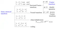
Relation
From the following picture, we summarize the LCT with other transform or properties
In optics and quantum mechanics
Paraxial optical systems implemented entirely with thin lenses and propagation through free space and/or graded index (GRIN) media, are quadratic phase systems (QPS); these were known before Moshinsky and Quesne (1974) called attention to their significance in connection with canonical transformations in quantum mechanics. The effect of any arbitrary QPS on an input wavefield can be described using the linear canonical transform, a particular case of which was developed by Segal (1963) and Bargmann (1961) in order to formalize Fock's (1928) boson calculus.[3]
In Quantum mechanics, linear canonical transformations can be identified with the linear transformations which mix the Momentum operator with the Position operator and leave invariant the Canonical commutation relations.
Applications
Canonical transforms are used to analyze differential equations. These include diffusion, the Schrödinger free particle, the linear potential (free-fall), and the attractive and repulsive oscillator equations. It also includes a few others such as the Fokker–Planck equation. Although this class is far from universal, the ease with which solutions and properties are found makes canonical transforms an attractive tool for problems such as these.[4]
Wave propagation through air, a lens, and between satellite dishes are discussed here. All of the computations can be reduced to 2×2 matrix algebra. This is the spirit of LCT.
Electromagnetic wave propagation
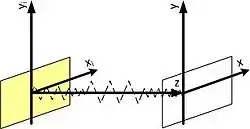
Assuming the system looks like as depicted in the figure, the wave travels from plane xi, yi to the plane of x and y.
The Fresnel transform is used to describe electromagnetic wave propagation in air:

with
k = 2 π / λ : wave number; λ : wavelength; z : distance of propagation; j : imaginary unit.
This is equivalent to LCT (shearing), when
When the travel distance (z) is larger, the shearing effect is larger.
Spherical lens
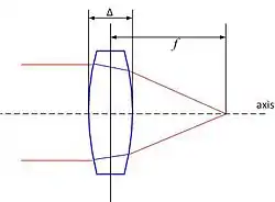
With the lens as depicted in the figure, and the refractive index denoted as n, the result is:[5]

with f the focal length and Δ the thickness of the lens.
The distortion passing through the lens is similar to LCT, when

This is also a shearing effect: when the focal length is smaller, the shearing effect is larger.
Spherical Mirror
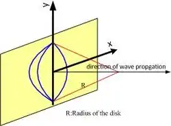
The spherical mirror—e.g., a satellite dish—can be described as a LCT, with

This is very similar to lens, except focal length is replaced by the radius of the dish. Therefore, if the radius is smaller, the shearing effect is larger.
Joint Free space and Spherical lens
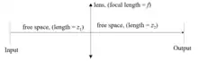
The relation between the input and output we can use LCT to represent

(1) If z1 = z2 = 2f, it is reverse real image
(2) If z1 = z2 = f, it is Fourier transform+scaling
(3) if z1=z2, it is fractional Fourier transform+scaling
Basic Properties
In this part, we show the basic properties of LCT
| Operator | Matrix of transform |
|---|---|


With the two-dimension column vector r defined as r =, we show some basic properties (result) for the specific input below

| Input | Output | Remark |
|---|---|---|
| Linearity | ||
| parseval's theorem | ||
| complex conjugate | ||
| multiplication | ||
| derivation | ||
| modulation | ||
| shift | ||
| scaling | ||
| scaling | ||
| 1 | ||


Example
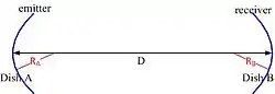
The system considered is depicted in the figure to the right: two dishes – one being the emitter and the other one the receiver – and a signal travelling between them over a distance D. First, for dish A (emitter), the LCT matrix looks like this:

Then, for dish B (receiver), the LCT matrix similarly becomes:

Last, for the propagation of the signal in air, the LCT matrix is:

Putting all three components together, the LCT of the system is:

Relation with Particle physics
It has been shown that it may be possible to establish a relation between some properties of the elementary Fermion in the Standard Model of Particle physics and Spin representation of linear canonical transformations. [6] In this approach, the Electric charge, Weak hypercharge and Weak isospin of the particles are expressed as linear combinations of some operators defined from the generators of the Clifford algebra associated with the spin representation of linear canonical transformations.
See also
- Segal–Shale–Weil distribution, a metaplectic group of operators related to the chirplet transform
- Other time–frequency transforms
- Applications
Notes
- de Bruijn, N. G. (1973). "A theory of generalized functions, with applications to Wigner distribution and Weyl correspondence", Nieuw Arch. Wiskd., III. Ser., 21 205-280.
- P.R. Deshmukh & A.S. Gudadhe (2011) Convolution structure for two version of fractional Laplace transform. Journal of Science and Arts, 2(15):143-150. "Archived copy". Archived from the original on 2012-12-23. Retrieved 2012-08-29.CS1 maint: archived copy as title (link)
- K.B. Wolf (1979) Ch. 9:Canonical transforms.
- K.B. Wolf (1979) Ch. 9 & 10.
- Goodman, Joseph W. (2005), Introduction to Fourier optics (3rd ed.), Roberts and Company Publishers, ISBN 0-9747077-2-4, §5.1.3, pp. 100–102.
- R. T. Ranaivoson, Raoelina Andriambololona, R. Hanitriarivo, R. Raboanary (2020). https://arxiv.org/abs/1804.10053
References
- J.J. Healy, M.A. Kutay, H.M. Ozaktas and J.T. Sheridan, "Linear Canonical Transforms: Theory and Applications", Springer, New York 2016.
- J.J. Ding, "Time–frequency analysis and wavelet transform course note", the Department of Electrical Engineering, National Taiwan University (NTU), Taipei, Taiwan, 2007.
- K.B. Wolf, "Integral Transforms in Science and Engineering", Ch. 9&10, New York, Plenum Press, 1979.
- S.A. Collins, "Lens-system diffraction integral written in terms of matrix optics," J. Opt. Soc. Amer. 60, 1168–1177 (1970).
- M. Moshinsky and C. Quesne, "Linear canonical transformations and their unitary representations," J. Math. Phys. 12, 8, 1772–1783, (1971).
- B.M. Hennelly and J.T. Sheridan, "Fast Numerical Algorithm for the Linear Canonical Transform", J. Opt. Soc. Am. A 22, 5, 928–937 (2005).
- H.M. Ozaktas, A. Koç, I. Sari, and M.A. Kutay, "Efficient computation of quadratic-phase integrals in optics", Opt. Let. 31, 35–37, (2006).
- Bing-Zhao Li, Ran Tao, Yue Wang, "New sampling formulae related to the linear canonical transform", Signal Processing '87', 983–990, (2007).
- A. Koç, H.M. Ozaktas, C. Candan, and M.A. Kutay, "Digital computation of linear canonical transforms", IEEE Trans. Signal Process., vol. 56, no. 6, 2383–2394, (2008).
- Ran Tao, Bing-Zhao Li, Yue Wang, "On sampling of bandlimited signals associated with the linear canonical transform", IEEE Transactions on Signal Processing, vol. 56, no. 11, 5454–5464, (2008).
- D. Stoler, "Operator methods in Physical Optics", 26th Annual Technical Symposium. International Society for Optics and Photonics, 1982.
- Tian-Zhou Xu, Bing-Zhao Li, " Linear Canonical Transform and Its Applications ", Beijing, Science Press, 2013.
- Raoelina Andriambololona, R. T. Ranaivoson, H.D.E Randriamisy, R. Hanitriarivo, "Dispersion Operators Algebra and Linear Canonical Transformations",International Journal of Theoretical Physics, Volume 56, Issue 4, pp 1258–1273, Springer, 2017
- R.T. Ranaivoson, Raoelina Andriambololona, R. Hanitriarivo, R. Raboanary "Linear Canonical Transformations in Relativistic Quantum Physics",arXiv:1804.10053 [quant-ph], 2020.
- Tatiana Alieva., Martin J. Bastiaans. (2016) The Linear Canonical Transformations: Definition and Properties. In: Healy J., Alper Kutay M., Ozaktas H., Sheridan J. (eds) Linear Canonical Transforms. Springer Series in Optical Sciences, vol 198. Springer, New York, NY
