Linear form
In mathematics, a linear form (also known as a linear functional,[1] a one-form, or a covector) is a linear map from a vector space to its field of scalars (often, the real numbers or the complex numbers).
If V is a vector space over a field k, the set of all linear functionals from V to k is itself a vector space over k with addition and scalar multiplication defined pointwise. This space is called the dual space of V, or sometimes the algebraic dual space, when a topological dual space is also considered. It is often denoted Hom(V, k),[2] or, when the field is understood, ;[3] other notations are also used, such as ,[4][5] or [2] When vectors are represented by column vectors (as it is common when a basis is fixed), then linear functionals are represented as row vectors, and their values on specific vectors are given by matrix products (with the row vector on the left).


Examples
The "constant zero function," mapping every vector to zero, is trivially a linear functional. Every other linear functional (such as the ones below) is surjective (i.e. its range is all of k).
Linear functionals in Rn
Suppose that vectors in the real coordinate space Rn are represented as column vectors

For each row vector [a1 ⋯ an] there is a linear functional f defined by

and each linear functional can be expressed in this form.
This can be interpreted as either the matrix product or the dot product of the row vector [a1 ⋯ an] and the column vector :


(Definite) Integration
Linear functionals first appeared in functional analysis, the study of vector spaces of functions. A typical example of a linear functional is integration: the linear transformation defined by the Riemann integral

is a linear functional from the vector space C[a, b] of continuous functions on the interval [a, b] to the real numbers. The linearity of I follows from the standard facts about the integral:

Evaluation
Let Pn denote the vector space of real-valued polynomial functions of degree ≤n defined on an interval [a, b]. If c ∈ [a, b], then let evc : Pn → R be the evaluation functional

The mapping f → f(c) is linear since

If x0, ..., xn are n + 1 distinct points in [a, b], then the evaluation functionals evxi, i = 0, 1, ..., n form a basis of the dual space of Pn. (Lax (1996) proves this last fact using Lagrange interpolation.)
Non-example
A function f having the equation of a line f(x) = a + rx with a ≠ 0 (e.g. f(x) = 1 + 2x) is not a linear functional on ℝ, since it is not linear.[nb 1] It is, however, affine-linear.
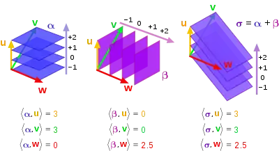
Visualization
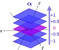
In finite dimensions, a linear functional can be visualized in terms of its level sets, the sets of vectors which map to a given value. In three dimensions, the level sets of a linear functional are a family of mutually parallel planes; in higher dimensions, they are parallel hyperplanes. This method of visualizing linear functionals is sometimes introduced in general relativity texts, such as Gravitation by Misner, Thorne & Wheeler (1973).
Applications
Application to quadrature
If x0, ..., xn are n + 1 distinct points in [a, b], then the linear functionals evxi : f → f(xi) defined above form a basis of the dual space of Pn, the space of polynomials of degree ≤ n. The integration functional I is also a linear functional on Pn, and so can be expressed as a linear combination of these basis elements. In symbols, there are coefficients a0, ..., an for which

for all f ∈ Pn. This forms the foundation of the theory of numerical quadrature.[6]
In quantum mechanics
Linear functionals are particularly important in quantum mechanics. Quantum mechanical systems are represented by Hilbert spaces, which are anti–isomorphic to their own dual spaces. A state of a quantum mechanical system can be identified with a linear functional. For more information see bra–ket notation.
Distributions
In the theory of generalized functions, certain kinds of generalized functions called distributions can be realized as linear functionals on spaces of test functions.
Dual vectors and bilinear forms
Every non-degenerate bilinear form on a finite-dimensional vector space V induces an isomorphism V → V∗ : v ↦ v∗ such that

where the bilinear form on V is denoted ⟨ , ⟩ (for instance, in Euclidean space ⟨v, w⟩ = v ⋅ w is the dot product of v and w).
The inverse isomorphism is V∗ → V : v∗ ↦ v, where v is the unique element of V such that

The above defined vector v∗ ∈ V∗ is said to be the dual vector of v ∈ V.
In an infinite dimensional Hilbert space, analogous results hold by the Riesz representation theorem. There is a mapping V → V∗ into the continuous dual space V∗.
Relationship to bases
Basis of the dual space
Let the vector space V have a basis , not necessarily orthogonal. Then the dual space V* has a basis called the dual basis defined by the special property that


Or, more succinctly,

where δ is the Kronecker delta. Here the superscripts of the basis functionals are not exponents but are instead contravariant indices.
A linear functional belonging to the dual space can be expressed as a linear combination of basis functionals, with coefficients ("components") ui,


Then, applying the functional to a basis vector ej yields

due to linearity of scalar multiples of functionals and pointwise linearity of sums of functionals. Then

So each component of a linear functional can be extracted by applying the functional to the corresponding basis vector.
The dual basis and inner product
When the space V carries an inner product, then it is possible to write explicitly a formula for the dual basis of a given basis. Let V have (not necessarily orthogonal) basis . In three dimensions (n = 3), the dual basis can be written explicitly


for i = 1, 2, 3, where ε is the Levi-Civita symbol and the inner product (or dot product) on V.

In higher dimensions, this generalizes as follows

where is the Hodge star operator.

In abstract algebra
In abstract algebra, the notion of vector spaces is generalized to that of modules over a ring, which removes the restriction that coordinates must be divisible. Given a module M over the ring R, a linear form on M is a linear map from M to R, where the latter is considered as a module over itself. Equivalently, the space of linear forms is always precisely Homk(V,k), whether k is a field or not.
The existence of "enough" linear forms on a module is equivalent to projectivity.[8]
Dual Basis Lemma — An R-[[module (mathematics)|]] M is projective if and only if there exists a sequence {ai}i∈I ∈ MI and linear forms {fi}i∈ I such that, for any a ∈ M,

and the sum is well-defined because only finitely-many terms are nonzero.
Change of field
Any vector space X over ℂ is also a vector space over ℝ, endowed with a complex structure; that is, there exists a real vector subspace Xℝ such that we can (formally) write X = Xℝ ⊕ Xℝi as ℝ-vector spaces. Every ℂ-linear functional on X is a ℝ-linear operator, but it is not an ℝ-linear functional on X, because its range (namely, ℂ) is 2-dimensional over ℝ. (Conversely, a ℝ-linear functional has range too small to be a ℂ-linear functional as well.)
However, every ℂ-linear functional uniquely determines an ℝ-linear functional on Xℝ by restriction. More surprisingly, this result can be reversed: every ℝ-linear functional g on X induces a canonical ℂ-linear functional Lg ∈ X#, such that the real part of Lg is g: define
- Lg(x) := g(x) - i g(ix) for all x ∈ X.
L • is ℝ-linear (i.e. Lg+h = Lg + Lh and Lrg = r Lg for all r ∈ ℝ and g, h ∈ Xℝ#). Similarly, the inverse of the surjection Hom(X,ℂ) → Hom(X,ℝ) defined by f ↦ Im f is the map I ↦ (x ↦ I(ix) + i I(x)).
This relationship was discovered by Henry Löwig in 1934 (although it is usually credited to F. Murray),[9] and can be generalized to arbitrary finite extensions of a field in the natural way.
In infinite dimensions
Below, all vector spaces are over either the real numbers ℝ or the complex numbers ℂ.
If V is a topological vector space, the space of continuous linear functionals — the continuous dual — is often simply called the dual space. If V is a Banach space, then so is its (continuous) dual. To distinguish the ordinary dual space from the continuous dual space, the former is sometimes called the algebraic dual space. In finite dimensions, every linear functional is continuous, so the continuous dual is the same as the algebraic dual, but in infinite dimensions the continuous dual is a proper subspace of the algebraic dual.
A linear functional f on a (not necessarily locally convex) topological vector space X is continuous if and only if there exists a continuous seminorm p on X such that |f| ≤ p.[10]
Characterizing closed subspaces
Continuous linear functionals have nice properties for analysis: a linear functional is continuous if and only if its kernel is closed,[11] and a non-trivial continuous linear functional is an open map, even if the (topological) vector space is not complete.[12]
Hyperplanes and maximal subspaces
A vector subspace M of X is called maximal if M ⊊ X, but there are no vector subspaces N satisfying M ⊊ N ⊊ X. M is maximal if and only if it is the kernel of some non-trivial linear functional on X (i.e. M = ker f for some non-trivial linear functional f on X). A hyperplane in X is a translate of a maximal vector subspace. By linearity, a subset H of X is a hyperplane if and only if there exists some non-trivial linear functional f on X such that H = { x ∈ X : f(x) = 1}.[9]
Relationships between multiple linear functionals
Any two linear functionals with the same kernel are proportional (i.e. scalar multiples of each other). This fact can be generalized to the following theorem.
Theorem[13][14] — If f, g1, ..., gn are linear functionals on X, then the following are equivalent:
- f can be written as a linear combination of g1, ..., gn (i.e. there exist scalars s1, ..., sn such that f = s1 g1 + ⋅⋅⋅ + sn gn);
- ∩n
i=1 Ker gi ⊆ Ker f; - there exists a real number r such that |f(x)| ≤ r |gi(x)| for all x ∈ X and all i.
If f is a non-trivial linear functional on X with kernel N, x ∈ X satisfies f(x) = 1, and U is a balanced subset of X, then N ∩ (x + U) = ∅ if and only if |f(u)| < 1 for all u ∈ U.[12]
Hahn-Banach theorem
Any (algebraic) linear functional on a vector subspace can be extended to the whole space; for example, the evaluation functionals described above can be extended to the vector space of polynomials on all of ℝ. However, this extension cannot always be done while keeping the linear functional continuous. The Hahn-Banach family of theorems gives conditions under which this extension can be done. For example,
Hahn–Banach dominated extension theorem[15](Rudin 1991, Th. 3.2) — If p : X → ℝ is a sublinear function, and f : M → ℝ is a linear functional on a linear subspace M ⊆ X which is dominated by p on M, then there exists a linear extension F : X → ℝ of f to the whole space X that is dominated by p, i.e., there exists a linear functional F such that
- F(m) = f(m) for all m ∈ M,
- |F(x)| ≤ p(x) for all x ∈ X.
Equicontinuity of families of linear functionals
Let X be a topological vector space (TVS) with continuous dual space X'.
For any subset H of X', the following are equivalent:[16]
- H is equicontinuous;
- H is contained in the polar of some neighborhood of 0 in X;
- the (pre)polar of H is a neighborhood of 0 in X;
If H is an equicontinuous subset of X' then the following sets are also equicontinuous: the weak-* closure, the balanced hull, the convex hull, and the convex balanced hull.[16] Moreover, Alaoglu's theorem implies that the weak-* closure of an equicontinuous subset of X' is weak-* compact (and thus that every equicontinuous subset weak-* relatively compact).[17][16]
See also
- Discontinuous linear map
- Locally convex topological vector space – A vector space with a topology defined by convex open sets
- Positive linear functional
- Multilinear form – Map from multiple vectors to an underlying field of scalars, linear in each argument
- Topological vector space – Vector space with a notion of nearness
Notes
- For instance, f(1 + 1) = a + 2r ≠ 2a + 2r = f(1) + f(1).
References
- Axler (2015) p. 101, §3.92
- Tu (2011) p. 19, §3.1
- Katznelson & Katznelson (2008) p. 37, §2.1.3
- Axler (2015) p. 101, §3.94
- Halmos (1974) p. 20, §13
- Lax 1996
- Misner, Thorne & Wheeler (1973) p. 57
- Clark, Pete L. Commutative Algebra (PDF). Unpublished. Lemma 3.12.
- Narici & Beckenstein 2011, pp. 10-11.
- Narici & Beckenstein 2011, p. 126.
- Rudin 1991, Theorem 1.18
- Narici & Beckenstein 2011, p. 128.
- Rudin 1991, pp. 63-64.
- Narici & Beckenstein 2011, pp. 1-18.
- Narici & Beckenstein 2011, pp. 177-220.
- Narici & Beckenstein 2011, pp. 225-273.
- Schaefer & Wolff 1999, Corollary 4.3.
Bibliography
- Axler, Sheldon (2015), Linear Algebra Done Right, Undergraduate Texts in Mathematics (3rd ed.), Springer, ISBN 978-3-319-11079-0
- Bishop, Richard; Goldberg, Samuel (1980), "Chapter 4", Tensor Analysis on Manifolds, Dover Publications, ISBN 0-486-64039-6
- Conway, John B. (1990). A Course in Functional Analysis. Graduate Texts in Mathematics. 96 (2nd ed.). Springer. ISBN 0-387-97245-5.
- Dunford, Nelson (1988). Linear operators (in Romanian). New York: Interscience Publishers. ISBN 0-471-60848-3. OCLC 18412261.
- Halmos, Paul Richard (1974), Finite-Dimensional Vector Spaces, Undergraduate Texts in Mathematics (1958 2nd ed.), Springer, ISBN 0-387-90093-4
- Katznelson, Yitzhak; Katznelson, Yonatan R. (2008), A (Terse) Introduction to Linear Algebra, American Mathematical Society, ISBN 978-0-8218-4419-9
- Lax, Peter (1996), Linear algebra, Wiley-Interscience, ISBN 978-0-471-11111-5
- Misner, Charles W.; Thorne, Kip S.; Wheeler, John A. (1973), Gravitation, W. H. Freeman, ISBN 0-7167-0344-0
- Narici, Lawrence; Beckenstein, Edward (2011). Topological Vector Spaces. Pure and applied mathematics (Second ed.). Boca Raton, FL: CRC Press. ISBN 978-1584888666. OCLC 144216834.
- Rudin, Walter (1991). Functional Analysis. International Series in Pure and Applied Mathematics. 8 (Second ed.). New York, NY: McGraw-Hill Science/Engineering/Math. ISBN 978-0-07-054236-5. OCLC 21163277.
- Schaefer, Helmut H.; Wolff, Manfred P. (1999). Topological Vector Spaces. GTM. 8 (Second ed.). New York, NY: Springer New York Imprint Springer. ISBN 978-1-4612-7155-0. OCLC 840278135.
- Schutz, Bernard (1985), "Chapter 3", A first course in general relativity, Cambridge, UK: Cambridge University Press, ISBN 0-521-27703-5
- Trèves, François (2006) [1967]. Topological Vector Spaces, Distributions and Kernels. Mineola, N.Y.: Dover Publications. ISBN 978-0-486-45352-1. OCLC 853623322.
- Tu, Loring W. (2011), An Introduction to Manifolds, Universitext (2nd ed.), Springer, ISBN 978-0-8218-4419-9
- Wilansky, Albert (2013). Modern Methods in Topological Vector Spaces. Mineola, New York: Dover Publications, Inc. ISBN 978-0-486-49353-4. OCLC 849801114.
