AD–AS model
The AD–AS or aggregate demand–aggregate supply model is a macroeconomic model that explains price level and output through the relationship of aggregate demand and aggregate supply.

| Part of a series on |
| Macroeconomics |
|---|
 |
|
It is based on the theory of John Maynard Keynes presented in his work The General Theory of Employment, Interest and Money. It is one of the primary simplified representations in the modern field of macroeconomics, and is used by a broad array of economists, from libertarian, monetarist supporters of laissez-faire, such as Milton Friedman, to post-Keynesian supporters of economic interventionism, such as Joan Robinson.
Modeling
The AD/AS model is used to illustrate the Keynesian model of the business cycle. Movements of the two curves can be used to predict the effects that various exogenous events will have on two variables: real GDP and the price level. Furthermore, the model can be incorporated as a component in any of a variety of dynamic models (models of how variables like the price level and others evolve over time). The AD–AS model can be related to the Phillips curve model of wage or price inflation and unemployment. A special case is a horizontal AS curve which means the price level is constant. The AD curve represents the locus of equilibrium in the IS–LM model. The two models produce the same results with a constant price level.
Aggregate demand curve
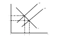
The AD (aggregate demand) curve is defined by the IS–LM equilibrium income at different potential price levels. The downward sloping AD curve is derived from the IS–LM model.

.png.webp)
It shows the combinations of the price level and level of the output at which the goods and assets markets are simultaneously in equilibrium.
The equation for the AD curve in general terms is:
where Y is real GDP, M is the nominal money supply, P is the price level, G is real government spending, T is real taxes levied, and Z1 other variables that affect the location of the IS curve (any component of spending) or the LM curve (influences on money demand). The real money supply has a positive effect on aggregate demand, as does real government spending; taxes has a negative effect on it.
Slope of AD curve
The slope of the AD curve reflects the extent to which real balances (i.e., the real value of the money balances held by an individual or by the economy as a whole) change the level of spending (consumption, government, investment), taking both assets and goods markets into consideration.
An increase in real balances will lead to an increase in equilibrium spending and income. These increases will be dependent on the value of the multiplier. For example, the smaller the interest responsiveness of money demand, the smaller the effect on spending and income; the higher the interest responsiveness of investment demand, the greater the resulting increase in spending and income.
Effect of monetary expansion on the AD curve

An increase in the nominal money stock leads to a higher real money stock at each level of prices. In the asset market, the decrease in interest rates induces the public to hold higher real balances. It stimulates the aggregate demand and thereby increases the equilibrium level of income and spending. Thus, the aggregate demand curve shifts right.
Aggregate supply curve
The aggregate supply curve (AS curve) describes the quantity of output the firms plan to supply for each given price level.
The Keynesian aggregate supply curve shows that the AS curve is significantly horizontal implying that the firm will supply whatever amount of goods is demanded at a particular price level during an economic depression. The idea behind that is because there is unemployment, firms can readily obtain as much labour as they want at that current wage and production can increase without any additional costs (e.g. machines are idle which can simply be turned on). Firms' average costs of production therefore are assumed not to change as their output level changes. This provides a rationale for Keynesians' support for government intervention. The total output of an economy can decline without the price level declining; this fact, in conjunction with the Keynesian belief of wages being inflexible downwards, clarifies the need for government stimulus. Since wages cannot readily adjust low enough for aggregate supply to shift outward and improve total output, the government must intervene to accomplish this result. However, the Keynesian aggregate supply curve also contains a normally upward-sloping region where aggregate supply responds accordingly to changes in price level. The upward slope is due to the law of diminishing returns as firms increase output, which states that it will become marginally more expensive to accomplish the same level of improvement in productive capacity as firms grow. It is also due to the scarcity of natural resources, the rarity of which causes increased production to also become more expensive. The vertical section of the Keynesian curve corresponds to the physical limit of the economy, where it is impossible to increase output.
The classical aggregate supply curve comprises a short-run aggregate supply curve and a vertical long-run aggregate supply curve. The short-run curve visualizes the total planned output of goods and services in the economy at a particular price level. The "short-run" is defined as the period during which only final good prices adjust and factor, or input, costs do not. The "long-run" is the period after which factor prices are able to adjust accordingly. The short-run aggregate supply curve has an upward slope for the same reasons the Keynesian AS curve has one: the law of diminishing returns and the scarcity of resources. The long-run aggregate supply curve is vertical because factor prices will have adjusted. Factor prices increase if producing at a point beyond full employment output, shifting the short-run aggregate supply inwards so equilibrium occurs somewhere along full employment output. Monetarists have argued that demand-side expansionary policies favoured by Keynesian economists are solely inflationary. As the aggregate demand curve is shifted outward, the general price level increases. This increased price level causes households, or the owners of the factors of production to demand higher prices for their goods and services. The consequence of this is increased production costs for firms, causing short-run aggregate demand to shift back inwards. The theoretical ultimate result is inflation.[1]
The mainstream AS-AD model contains both a long-run aggregate supply curve (LRAS) and a short-run aggregate supply (SRAS) curve essentially combining the classical and Keynesian models. In the short run wages and other resource prices are sticky and slow to adjust to new price levels. This gives way to the upward sloping SRAS. In the long-run, resource prices adjust to the price level bringing the economy back to a full employment output; along vertical LRAS.[2]
Shifts in aggregate supply curves
The Keynesian model, in which there is no long-run aggregate supply curve and the classical model, in the case of the short-run aggregate supply curve, are affected by the same determinants. Any event that results in a change of production costs shifts the curves outwards or inwards if production costs are decreased or increased, respectively. Some factors which affect short-run production costs include: taxes and subsidies, price of labour (wages), and price of raw materials. These factors shift short-run curves exclusively. Changes in the quantity and quality of labour and capital affect both long-run and short-run supply curves. A greater quantity of labour or capital corresponds to a lower price for both. A greater quality in labour or capital corresponds to a greater output per worker or machine.
The long-run aggregate supply curve of the classical model is affected by events that affect the potential output of the economy. Factors revolve around changes in the quality and quantity of factors of production.
Fiscal and monetary policy under Classical and Keynesian cases
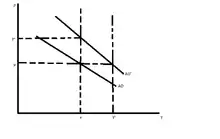
Keynesian Case: If there is a fiscal expansion i.e. there is an increase in the government spending or a cut in the taxes, it will shift the AD curve rightwards. The shift would then imply an increase in the equilibrium output and employment.
In the Classical case, the AS curve is vertical at the full employment level of output. Firms will supply the equilibrium level of output whatever the price level may be.
Now, the fiscal expansion shifts the AD curve rightwards, thus leading to an increase in the demand for goods, but the firms cannot increase the output as there is no labour force which can be obtained. As firms try to hire more labour, they bid up wages and their costs of production and thus they charge higher prices for the output. The increase in prices reduces the real money stock and leads to an increase in the interest rates and reduction in spending.
The equation for the aggregate supply curve in general terms for the case of excess supply in the labor market, called the short-run aggregate supply curve, is
where W is the nominal wage rate (exogenous due to stickiness in the short run), Pe is the anticipated (expected) price level, and Z2 is a vector of exogenous variables that can affect the position of the labor demand curve (the capital stock or the current state of technological knowledge). The real wage has a negative effect on firms' employment of labor and hence on aggregate supply. The price level relative to its expected level has a positive effect on aggregate supply because of firms' mistakes in production plans due to mis-predictions of prices.
The long-run aggregate supply curve refers not to a time frame in which the capital stock is free to be set optimally (as would be the terminology in the micro-economic theory of the firm), but rather to a time frame in which wages are free to adjust in order to equilibrate the labor market and in which price anticipations are accurate. In this case the nominal wage rate is endogenous and so does not appear as an independent variable in the aggregate supply equation. The long-run aggregate supply equation is simply
and is vertical at the full-employment level of output. In this long-run case, Z2 also includes factors affecting the position of the labor supply curve (such as population), since in labor market equilibrium the location of labor supply affects the labor market outcome.
Shifts of aggregate demand and aggregate supply
The following summarizes the exogenous events that could shift the aggregate supply or aggregate demand curve to the right. Exogenous events happening in the opposite direction would shift the relevant curve in the opposite direction.
Shifts of aggregate demand
The following exogenous events would shift the aggregate demand curve to the right. As a result, the price level would go up. In addition if the time frame of analysis is the short run, so the aggregate supply curve is upward sloping rather than vertical, real output would go up; but in the long run with aggregate supply vertical at full employment, real output would remain unchanged.
Rightward aggregate demand shifts emanating from the IS curve:
- An exogenous increase in consumer spending
- An exogenous increase in investment spending on physical capital
- An exogenous increase in intended inventory investment
- An exogenous increase in government spending on goods and services
- An exogenous increase in transfer payments from the government to the people
- An exogenous decrease in taxes levied
- An exogenous increase in purchases of the country's exports by people in other countries
- An exogenous decrease in imports from other countries
Rightward aggregate demand shifts emanating from the LM curve:
- An exogenous increase in the nominal money supply
- An exogenous increase in the demand for money supply i.e. liquidity preference
Shifts of aggregate supply
The following exogenous events would shift the short-run aggregate supply curve to the right. As a result, the price level would drop and real GDP would increase.
- An exogenous decrease in the wage rate
- An increase in the physical capital stock
- Technological progress — improvements in our knowledge of how to transform capital and labor into output
The following events would shift the long-run aggregate supply curve to the right:
- An increase in population
- An increase in the physical capital stock
- Technological progress
Transition dynamics
- Movement back to the steady state is fastest when the economy is furthest from its steady state.
- This means that as the aggregate supply is shocked by factors of production, it will move away from its steady state. In response, the supply will slowly shift back to the steady state equilibrium, first with a large reaction, then consequently smaller reactions until it reaches steady state. The reactions back to equilibrium are largest when furthest from steady state, and become smaller as they near equilibrium.
For example, a shock increase in the price of oil is felt by producers as an increase in the factors of production. This shifts the supply curve upward by raising expected inflation. This slows the adjustment of the AS curve back to its steady state. As the inflation slowly falls, so will the AS curve back to its steady state.
Monetarism
The modern quantity theory states that the price level is directly affected by the quantity of money. Milton Friedman was the recognized intellectual leader of an influential group of economists, called monetarists, who emphasize the role of money and monetary policy in affecting the behaviour of output and prices. The modern quantity theory also disagrees with the strict quantity theory in not believing that the supply curve is vertical in the short run. Thus, Friedman and other monetarists made an important distinction between the short run and long run effects of changes in money. They said that in the long run money is more or less neutral: changes in the nominal money stock have no real effects and only change prices. But in the short run, they argue that monetary policy and changes in the money stock can have important real effects.
References
- Glanville, Alan (2011). Economics From a Global Perspective (Third ed.). Glanville Books. p. 224. ISBN 9780952474685.
- Reed, Jacob (2016). "AP Macroeconomics Review: AS-AD Model". APEconReview.com. Archived from the original on 25 June 2016. Retrieved 4 September 2020.
Further reading
- Blanchard, Olivier (2006). Macroeconomics (Fourth ed.). Pearson Education. ISBN 0-13-186026-7.
- Dutt, Amitava K.; Skott, Peter (1996). "Keynesian Theory and the Aggregate-Supply/Aggregate-Demand Framework: A Defense". Eastern Economic Journal. 22 (3): 313–331.
- Dutt, Amitava K.; Skott, Peter (2006). "Keynesian Theory and the AD-AS Framework: A Reconsideration". In Chiarella, Carl; Franke, Reiner; Flaschel, Peter; Semmler, Willi (eds.). Quantitative and Empirical Analysis of Nonlinear Dynamic Macromodels. Contributions to Economic Analysis. 277. Emerald Group. pp. 149–172. doi:10.1016/S0573-8555(05)77006-1.
- Mankiw, N. Gregory (2007). Macroeconomics (Sixth ed.). New York: Worth Publishers. ISBN 978-0-7167-6213-3.
- Palley, Thomas I. (1997). "Keynesian Theory and AS/AD Analysis". Eastern Economic Journal. 23 (4): 459–468. JSTOR 40325806.
External links
| Wikimedia Commons has media related to Aggregate supply and demand curves. |
- Sparknotes: Aggregate Supply and Aggregate Demand brief explanation of the AD–AS model
- "Aggregate Demand and Aggregate Supply" in CyberEconomics by Robert Schenk explains the AD–AS model and explains its relation to the IS/LM model
- "ThinkEconomics: Macroeconomic Phenomena in the AD/AS Model" includes an interactive graph demonstrating inflationary changes in a graph based on the AD–AS model
- "ThinkEconomics: The Aggregate Demand and Aggregate Supply Model" includes an interactive AD-AS graph that tests one's knowledge of how the AD and AS curves shift under different conditions
