List of map projections

Projection	Image	Type	Properties	Creator	Year	Notes
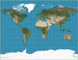
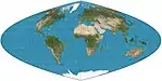
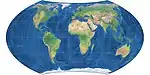
Equirectangular = equidistant cylindrical = rectangular = la carte parallélogrammatique		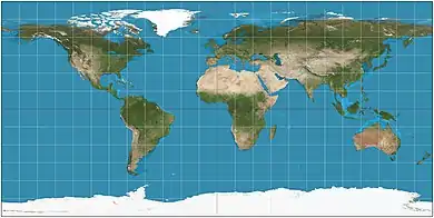Cylindrical	Equidistant	Marinus of Tyre	0120 c. 120	Simplest geometry; distances along meridians are conserved. Plate carrée: special case having the equator as the standard parallel.
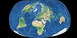
Cassini = Cassini–Soldner		Cylindrical	Equidistant	César-François Cassini de Thury	1745	Transverse of equidistant projection; distances along central meridian are conserved. Distances perpendicular to central meridian are preserved.
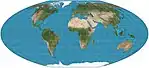
Mercator = Wright		Cylindrical	Conformal	Gerardus Mercator	1569	Lines of constant bearing (rhumb lines) are straight, aiding navigation. Areas inflate with latitude, becoming so extreme that the map cannot show the poles.
Web Mercator		Cylindrical	Compromise	Google	2005	Variant of Mercator that ignores Earth's ellipticity for fast calculation, and clips latitudes to ~85.05° for square presentation. De facto standard for Web mapping applications.
Gauss–Krüger = Gauss conformal = (ellipsoidal) transverse Mercator		Cylindrical	Conformal	Carl Friedrich Gauss Johann Heinrich Louis Krüger	1822	This transverse, ellipsoidal form of the Mercator is finite, unlike the equatorial Mercator. Forms the basis of the Universal Transverse Mercator coordinate system.
Roussilhe oblique stereographic				Henri Roussilhe	1922
Hotine oblique Mercator		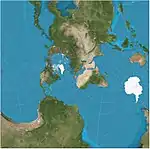Cylindrical	Conformal	M. Rosenmund, J. Laborde, Martin Hotine	1903
Gall stereographic		Cylindrical	Compromise	James Gall	1855	Intended to resemble the Mercator while also displaying the poles. Standard parallels at 45°N/S.
Miller = Miller cylindrical		Cylindrical	Compromise	Osborn Maitland Miller	1942	Intended to resemble the Mercator while also displaying the poles.
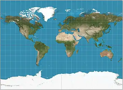
Lambert cylindrical equal-area		Cylindrical	Equal-area	Johann Heinrich Lambert	1772	Standard parallel at the equator. Aspect ratio of π (3.14). Base projection of the cylindrical equal-area family.
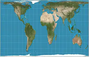
Behrmann		Cylindrical	Equal-area	Walter Behrmann	1910	Horizontally compressed version of the Lambert equal-area. Has standard parallels at 30°N/S and an aspect ratio of 2.36.
Hobo–Dyer		Cylindrical	Equal-area	Mick Dyer	2002	Horizontally compressed version of the Lambert equal-area. Very similar are Trystan Edwards and Smyth equal surface (= Craster rectangular) projections with standard parallels at around 37°N/S. Aspect ratio of ~2.0.
Gall–Peters = Gall orthographic = Peters		Cylindrical	Equal-area	James Gall (Arno Peters)	1855	Horizontally compressed version of the Lambert equal-area. Standard parallels at 45°N/S. Aspect ratio of ~1.6. Similar is Balthasart projection with standard parallels at 50°N/S.
Central cylindrical		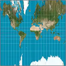Cylindrical	Perspective	(unknown)	1850 c. 1850	Practically unused in cartography because of severe polar distortion, but popular in panoramic photography, especially for architectural scenes.
Sinusoidal = Sanson–Flamsteed = Mercator equal-area		Pseudocylindrical	Equal-area, equidistant	(Several; first is unknown)	1600 c. 1600	Meridians are sinusoids; parallels are equally spaced. Aspect ratio of 2:1. Distances along parallels are conserved.
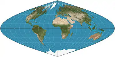
Mollweide = elliptical = Babinet = homolographic		Pseudocylindrical	Equal-area	Karl Brandan Mollweide	1805	Meridians are ellipses.
Eckert II		Pseudocylindrical	Equal-area	Max Eckert-Greifendorff	1906
Eckert IV		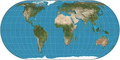Pseudocylindrical	Equal-area	Max Eckert-Greifendorff	1906	Parallels are unequal in spacing and scale; outer meridians are semicircles; other meridians are semiellipses.
Eckert VI		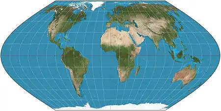Pseudocylindrical	Equal-area	Max Eckert-Greifendorff	1906	Parallels are unequal in spacing and scale; meridians are half-period sinusoids.
Ortelius oval		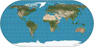Pseudocylindrical	Compromise	Battista Agnese	1540	Meridians are circular.[2]
Goode homolosine		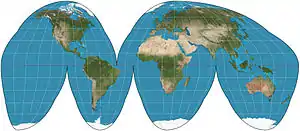Pseudocylindrical	Equal-area	John Paul Goode	1923	Hybrid of Sinusoidal and Mollweide projections. Usually used in interrupted form.
Kavrayskiy VII		Pseudocylindrical	Compromise	Vladimir V. Kavrayskiy	1939	Evenly spaced parallels. Equivalent to Wagner VI horizontally compressed by a factor of ${\displaystyle {\sqrt {3}}/{2}}$.
Robinson		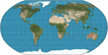Pseudocylindrical	Compromise	Arthur H. Robinson	1963	Computed by interpolation of tabulated values. Used by Rand McNally since inception and used by NGS in 1988–1998.
Equal Earth		Pseudocylindrical	Equal-area	Bojan Šavrič, Tom Patterson, Bernhard Jenny	2018	Inspired by the Robinson projection, but retains the relative size of areas.
Natural Earth		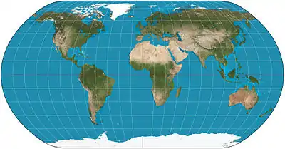Pseudocylindrical	Compromise	Tom Patterson	2011	Computed by interpolation of tabulated values.
Tobler hyperelliptical		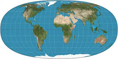Pseudocylindrical	Equal-area	Waldo R. Tobler	1973	A family of map projections that includes as special cases Mollweide projection, Collignon projection, and the various cylindrical equal-area projections.
Wagner VI		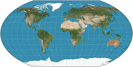Pseudocylindrical	Compromise	K. H. Wagner	1932	Equivalent to Kavrayskiy VII vertically compressed by a factor of ${\displaystyle {\sqrt {3}}/{2}}$.
Collignon		Pseudocylindrical	Equal-area	Édouard Collignon	1865 c. 1865	Depending on configuration, the projection also may map the sphere to a single diamond or a pair of squares.
HEALPix		Pseudocylindrical	Equal-area	Krzysztof M. Górski	1997	Hybrid of Collignon + Lambert cylindrical equal-area.
Boggs eumorphic		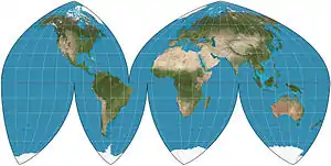Pseudocylindrical	Equal-area	Samuel Whittemore Boggs	1929	The equal-area projection that results from average of sinusoidal and Mollweide y-coordinates and thereby constraining the x coordinate.
Craster parabolic =Putniņš P4		Pseudocylindrical	Equal-area	John Craster	1929	Meridians are parabolas. Standard parallels at 36°46′N/S; parallels are unequal in spacing and scale; 2:1 aspect.
McBryde–Thomas flat-pole quartic = McBryde–Thomas #4		Pseudocylindrical	Equal-area	Felix W. McBryde, Paul Thomas	1949	Standard parallels at 33°45′N/S; parallels are unequal in spacing and scale; meridians are fourth-order curves. Distortion-free only where the standard parallels intersect the central meridian.
Quartic authalic		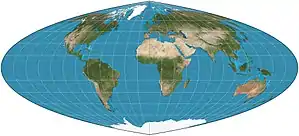Pseudocylindrical	Equal-area	Karl Siemon Oscar Adams	1937 1944	Parallels are unequal in spacing and scale. No distortion along the equator. Meridians are fourth-order curves.
The Times		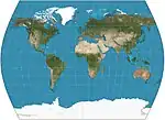Pseudocylindrical	Compromise	John Muir	1965	Standard parallels 45°N/S. Parallels based on Gall stereographic, but with curved meridians. Developed for Bartholomew Ltd., The Times Atlas.
Loximuthal		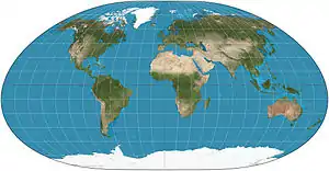Pseudocylindrical	Compromise	Karl Siemon Waldo R. Tobler	1935 1966	From the designated centre, lines of constant bearing (rhumb lines/loxodromes) are straight and have the correct length. Generally asymmetric about the equator.
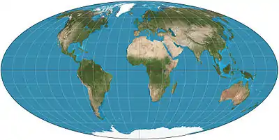
Aitoff		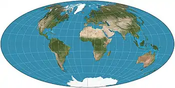Pseudoazimuthal	Compromise	David A. Aitoff	1889	Stretching of modified equatorial azimuthal equidistant map. Boundary is 2:1 ellipse. Largely superseded by Hammer.
Hammer = Hammer–Aitoff variations: Briesemeister; Nordic		Pseudoazimuthal	Equal-area	Ernst Hammer	1892	Modified from azimuthal equal-area equatorial map. Boundary is 2:1 ellipse. Variants are oblique versions, centred on 45°N.
Strebe 1995		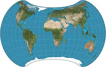Pseudoazimuthal	Equal-area	Daniel "daan" Strebe	1994	Formulated by using other equal-area map projections as transformations.
Winkel tripel		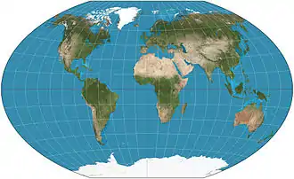Pseudoazimuthal	Compromise	Oswald Winkel	1921	Arithmetic mean of the equirectangular projection and the Aitoff projection. Standard world projection for the NGS since 1998.
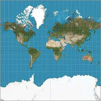
Van der Grinten		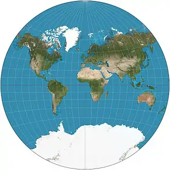Other	Compromise	Alphons J. van der Grinten	1904	Boundary is a circle. All parallels and meridians are circular arcs. Usually clipped near 80°N/S. Standard world projection of the NGS in 1922–1988.
Equidistant conic = simple conic		Conic	Equidistant	Based on Ptolemy's 1st Projection	0100 c. 100	Distances along meridians are conserved, as is distance along one or two standard parallels.[3]
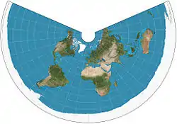
Lambert conformal conic		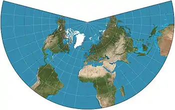Conic	Conformal	Johann Heinrich Lambert	1772	Used in aviation charts.
Albers conic		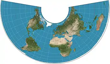Conic	Equal-area	Heinrich C. Albers	1805	Two standard parallels with low distortion between them.
Werner		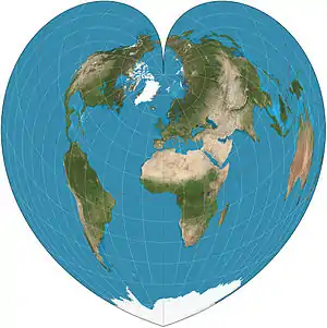Pseudoconical	Equal-area, equidistant	Johannes Stabius	1500 c. 1500	Parallels are equally spaced concentric circular arcs. Distances from the North Pole are correct as are the curved distances along parallels and distances along central meridian.
Bonne		Pseudoconical, cordiform	Equal-area	Bernardus Sylvanus	1511	Parallels are equally spaced concentric circular arcs and standard lines. Appearance depends on reference parallel. General case of both Werner and sinusoidal.
Bottomley		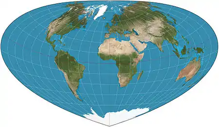Pseudoconical	Equal-area	Henry Bottomley	2003	Alternative to the Bonne projection with simpler overall shape Parallels are elliptical arcs Appearance depends on reference parallel.
American polyconic		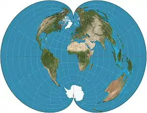Pseudoconical	Compromise	Ferdinand Rudolph Hassler	1820 c. 1820	Distances along the parallels are preserved as are distances along the central meridian.
Rectangular polyconic		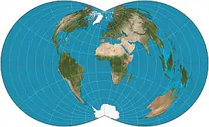Pseudoconical	Compromise	U.S. Coast Survey	1853 c. 1853	Latitude along which scale is correct can be chosen. Parallels meet meridians at right angles.
Latitudinally equal-differential polyconic		Pseudoconical	Compromise	China State Bureau of Surveying and Mapping	1963	Polyconic: parallels are non-concentric arcs of circles.
Nicolosi globular		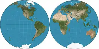Pseudoconical[4]	Compromise	Abū Rayḥān al-Bīrūnī; reinvented by Giovanni Battista Nicolosi, 1660.[1]:14	1000 c. 1000
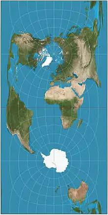
Azimuthal equidistant =Postel =zenithal equidistant		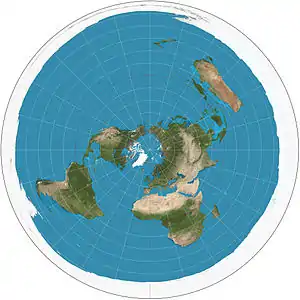Azimuthal	Equidistant	Abū Rayḥān al-Bīrūnī	1000 c. 1000	Distances from center are conserved. Used as the emblem of the United Nations, extending to 60° S.
Gnomonic		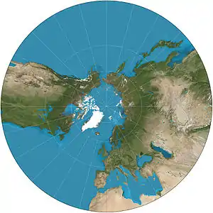Azimuthal	Gnomonic	Thales (possibly)	c. 580 BC	All great circles map to straight lines. Extreme distortion far from the center. Shows less than one hemisphere.
Lambert azimuthal equal-area		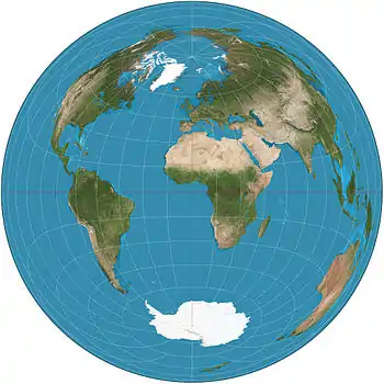Azimuthal	Equal-area	Johann Heinrich Lambert	1772	The straight-line distance between the central point on the map to any other point is the same as the straight-line 3D distance through the globe between the two points.
Stereographic		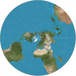Azimuthal	Conformal	Hipparchos*	c. 200 BC	Map is infinite in extent with outer hemisphere inflating severely, so it is often used as two hemispheres. Maps all small circles to circles, which is useful for planetary mapping to preserve the shapes of craters.
Orthographic		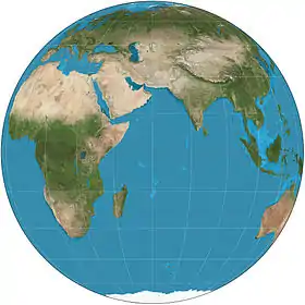Azimuthal	Perspective	Hipparchos*	c. 200 BC	View from an infinite distance.
Vertical perspective		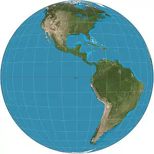Azimuthal	Perspective	Matthias Seutter*	1740	View from a finite distance. Can only display less than a hemisphere.
Two-point equidistant		Azimuthal	Equidistant	Hans Maurer	1919	Two "control points" can be almost arbitrarily chosen. The two straight-line distances from any point on the map to the two control points are correct.
Peirce quincuncial		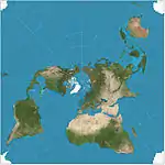Other	Conformal	Charles Sanders Peirce	1879	Tessellates. Can be tiled continuously on a plane, with edge-crossings matching except for four singular points per tile.
Guyou hemisphere-in-a-square projection		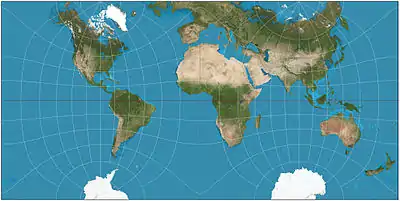Other	Conformal	Émile Guyou	1887	Tessellates.
Adams hemisphere-in-a-square projection		Other	Conformal	Oscar Sherman Adams	1925
Lee conformal world on a tetrahedron		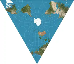Polyhedral	Conformal	L. P. Lee	1965	Projects the globe onto a regular tetrahedron. Tessellates.
Octant projection		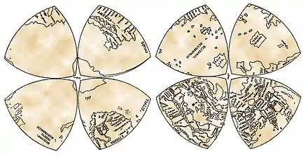Polyhedral	Compromise	Leonardo da Vinci	1514	Projects the globe onto eight octants (Reuleaux triangles) with no meridians and no parallels.
Cahill's butterfly map		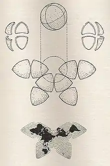Polyhedral	Compromise	Bernard Joseph Stanislaus Cahill	1909	Projects the globe onto an octahedron with symmetrical components and contiguous landmasses that may be displayed in various arrangements.
Cahill–Keyes projection		Polyhedral	Compromise	Gene Keyes	1975	Projects the globe onto a truncated octahedron with symmetrical components and contiguous land masses that may be displayed in various arrangements.
Waterman butterfly projection		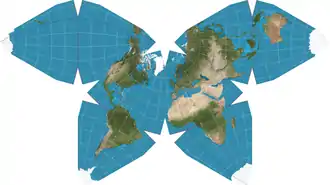Polyhedral	Compromise	Steve Waterman	1996	Projects the globe onto a truncated octahedron with symmetrical components and contiguous land masses that may be displayed in various arrangements.
Quadrilateralized spherical cube		Polyhedral	Equal-area	F. Kenneth Chan, E. M. O'Neill	1973
Dymaxion map		Polyhedral	Compromise	Buckminster Fuller	1943	Also known as a Fuller Projection.
AuthaGraph projection	Link to file	Polyhedral	Compromise	Hajime Narukawa	1999	Approximately equal-area. Tessellates.
Myriahedral projections		Polyhedral	Equal-area	Jarke J. van Wijk	2008	Projects the globe onto a myriahedron: a polyhedron with a very large number of faces.[5][6]
Craig retroazimuthal = Mecca		Retroazimuthal	Compromise	James Ireland Craig	1909
Hammer retroazimuthal, front hemisphere		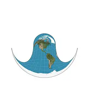Retroazimuthal		Ernst Hammer	1910
Hammer retroazimuthal, back hemisphere		Retroazimuthal		Ernst Hammer	1910
Littrow		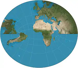Retroazimuthal	Conformal	Joseph Johann Littrow	1833	on equatorial aspect it shows a hemisphere except for poles.
Armadillo		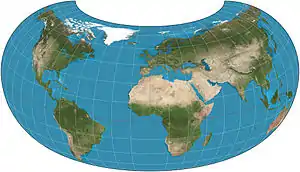Other	Compromise	Erwin Raisz	1943
GS50		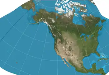Other	Conformal	John P. Snyder	1982	Designed specifically to minimize distortion when used to display all 50 U.S. states.
Wagner VII = Hammer-Wagner		Pseudoazimuthal	Equal-area	K. H. Wagner	1941
Atlantis = Transverse Mollweide		Pseudocylindrical	Equal-area	John Bartholomew	1948	Oblique version of Mollweide
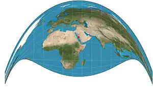
Bertin = Bertin-Rivière = Bertin 1953		Other	Compromise	Jacques Bertin	1953	Projection in which the compromise is no longer homogeneous but instead is modified for a larger deformation of the oceans, to achieve lesser deformation of the continents. Commonly used for French geopolitical maps.[7]

*The first known popularizer/user and not necessarily the creator.

• Snyder, John P. (1987). "Map projections: A working manual". Map projections – A working manual (PDF). U.S. Geological Survey Professional Paper. 1395. Washington, D.C.: U.S. Government Printing Office. doi:10.3133/pp1395. Retrieved 2019-02-18.
• Snyder, John P.; Voxland, Philip M. (1989). An Album of Map Projections (PDF). U.S. Geological Survey Professional Paper. 1453. Washington, D.C.: U.S. Government Printing Office. doi:10.3133/pp1453. Retrieved 2019-02-18.