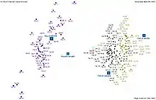
Biplot
Biplots are a type of exploratory graph used in statistics, a generalization of the simple two-variable scatterplot. A biplot allows information on both samples and variables of a data matrix to be displayed graphically. Samples are displayed as points while variables are displayed either as vectors, linear axes or nonlinear trajectories. In the case of categorical variables, category level points may be used to represent the levels of a categorical variable. A generalised biplot displays information on both continuous and categorical variables.


Introduction and history
The biplot was introduced by K. Ruben Gabriel (1971).[1] Gower and Hand (1996) wrote a monograph on biplots. Yan and Kang (2003) described various methods which can be used in order to visualize and interpret a biplot. The book by Greenacre (2010)[2] is a practical user-oriented guide to biplots, along with scripts in the open-source R programming language, to generate biplots associated with principal component analysis (PCA), multidimensional scaling (MDS), log-ratio analysis (LRA)—also known as spectral mapping[3][4]—discriminant analysis (DA) and various forms of correspondence analysis: simple correspondence analysis (CA), multiple correspondence analysis (MCA) and canonical correspondence analysis (CCA) (Greenacre 2016[5]). The book by Gower, Lubbe and le Roux (2011) aims to popularize biplots as a useful and reliable method for the visualization of multivariate data when researchers want to consider, for example, principal component analysis (PCA), canonical variates analysis (CVA) or various types of correspondence analysis.
Construction
A biplot is constructed by using the singular value decomposition (SVD) to obtain a low-rank approximation to a transformed version of the data matrix X, whose n rows are the samples (also called the cases, or objects), and whose p columns are the variables. The transformed data matrix Y is obtained from the original matrix X by centering and optionally standardizing the columns (the variables). Using the SVD, we can write Y = ∑k=1,...pdkukvkT;, where the uk are n-dimensional column vectors, the vk are p-dimensional column vectors, and the dk are a non-increasing sequence of non-negative scalars. The biplot is formed from two scatterplots that share a common set of axes and have a between-set scalar product interpretation. The first scatterplot is formed from the points (d1αu1i, d2αu2i), for i = 1,...,n. The second plot is formed from the points (d11−αv1j, d21−αv2j), for j = 1,...,p. This is the biplot formed by the dominant two terms of the SVD, which can then be represented in a two-dimensional display. Typical choices of α are 1 (to give a distance interpretation to the row display) and 0 (to give a distance interpretation to the column display), and in some rare cases α=1/2 to obtain a symmetrically scaled biplot (which gives no distance interpretation to the rows or the columns, but only the scalar product interpretation). The set of points depicting the variables can be drawn as arrows from the origin to reinforce the idea that they represent biplot axes onto which the samples can be projected to approximate the original data.
References
- 'Gabriel, K. R. (1971). The biplot graphic display of matrices with application to principal component analysis. Biometrika, 58(3), 453–467.
- Greenacre, M. (2010). Biplots in Practice. BBVA Foundation, Bilbao, Spain. Available for free at http://www.multivariatestatistics.org
- Lewi, Paul J. (2005). "Spectral mapping, a personal and historical account of an adventure in multivariate data analysis". Chemometrics and Intelligent Laboratory Systems. 77 (1–2): 215–223. doi:10.1016/j.chemolab.2004.07.010.
- David Livingstone (2009). A Practical Guide to Scientific Data Analysis. Chichester, John Wiley & Sons Ltd, 233–238. ISBN 978-0-470-85153-1
- Greenacre, M. (2016) Correspondence Analysis in Practice. Third Edition. Chapman and Hall / CRC Press.ISBN 978-84-923846-8-6
Sources
- Gabriel, K.R. (1971). "The biplot graphic display of matrices with application to principal component analysis". Biometrika. 58 (3): 453–467. doi:10.1093/biomet/58.3.453.
- Gower, J.C., Lubbe, S. and le Roux, N. (2010). Understanding Biplots. Wiley. ISBN 978-0-470-01255-0
- Gower, J.C. and Hand, D.J (1996). Biplots. Chapman & Hall, London, UK. ISBN 0-412-71630-5
- Yan, W. and Kang, M.S. (2003). GGE Biplot Analysis. CRC Press, Boca Raton, Florida. ISBN 0-8493-1338-4
- Demey, J.R., Vicente-Villardón, J.L., Galindo-Villardón, M.P. and Zambrano, A.Y. (2008). Identifying molecular markers associated with classification of genotypes by External Logistic Biplots. Bioinformatics. 24(24):2832–2838
