Dirac comb
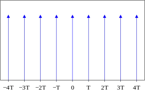
In mathematics, a Dirac comb (also known as an impulse train and sampling function in electrical engineering) is a periodic tempered distribution[1][2] constructed from Dirac delta functions

for some given period T. The symbol , where the period is omitted, represents a Dirac comb of unit period. Some authors, notably Bracewell, as well as some textbook authors in electrical engineering and circuit theory, refer to it as the Shah function (possibly because its graph resembles the shape of the Cyrillic letter sha Ш). Because the Dirac comb function is periodic, it can be represented as a Fourier series:


The Dirac comb function allows one to represent both continuous and discrete phenomena, such as sampling and aliasing, in a single framework of continuous Fourier analysis on Schwartz distributions, without any reference to Fourier series. Owing to the Poisson summation formula, in signal processing, the Dirac comb allows modelling sampling by multiplication with it, but it also allows modelling periodization by convolution with it.[3]
Dirac-comb identity
The Dirac comb can be constructed in two ways, either by using the comb operator (performing sampling) applied to the function that is constantly , or, alternatively, by using the rep operator (performing periodization) applied to the Dirac delta . Formally, this yields (Woodward 1953; Brandwood 2003)


where
- and


In signal processing, this property on one hand allows sampling a function by multiplication with , and on the other hand it also allows the periodization of by convolution with (Bracewell 1986). The Dirac comb identity is a particular case of the Convolution Theorem for tempered distributions.


Scaling
The scaling property of the Dirac comb follows from the properties of the Dirac delta function. Since [4] for positive real numbers , it follows that:


Note that requiring positive scaling numbers instead of negative ones is not a restriction because the negative sign would only reverse the order of the summation within , which does not affect the result.
Fourier series
It is clear that is periodic with period . That is,


for all t. The complex Fourier series for such a periodic function is

where the Fourier coefficients are (symbolically)

All Fourier coefficients are 1/T resulting in
When the period is one unit, this simplifies to

Remark: Most rigorously, Riemann or Lebesgue integration over any products including a Dirac delta function yields zero. For this reason, the integration above (Fourier series coefficients determination) must be understood "in the generalized functions sense". It means that, instead of using the characteristic function of an interval applied to the Dirac comb, one uses a so-called Lighthill unitary function as cutout function, see Lighthill 1958, p.62, Theorem 22 for details.
Fourier transform
The Fourier transform of a Dirac comb is also a Dirac comb. This is evident when one considers that all the Fourier components add constructively whenever is an integer multiple of .


Unitary transform to ordinary frequency domain (Hz):

Notably, the unit period Dirac comb transforms to itself:

The specific rule depends on the form of the Fourier transform used. When using a unitary transform of angular frequency (radian/s), the rule is

Sampling and aliasing
Multiplying any function by a Dirac comb transforms it into a train of impulses with integrals equal to the value of the function at the nodes of the comb. This operation is frequently used to represent sampling.

Due to the self-transforming property of the Dirac comb and the convolution theorem, this corresponds to convolution with the Dirac comb in the frequency domain.

Since convolution with a delta function is equivalent to shifting the function by , convolution with the Dirac comb corresponds to replication or periodic summation:


This leads to a natural formulation of the Nyquist–Shannon sampling theorem. If the spectrum of the function contains no frequencies higher than B (i.e., its spectrum is nonzero only in the interval ) then samples of the original function at intervals are sufficient to reconstruct the original signal. It suffices to multiply the spectrum of the sampled function by a suitable rectangle function, which is equivalent to applying a brick-wall lowpass filter.


In time domain, this "multiplication with the rect function" is equivalent to "convolution with the sinc function" (Woodward 1953, p.33-34). Hence, it restores the original function from its samples. This is known as the Whittaker–Shannon interpolation formula.
Remark: Most rigorously, multiplication of the rect function with a generalized function, such as the Dirac comb, fails. This is due to undetermined outcomes of the multiplication product at the interval boundaries. As a workaround, one uses a Lighthill unitary function instead of the rect function. It is smooth at the interval boundaries, hence it yields determined multiplication products everywhere, see Lighthill 1958, p.62, Theorem 22 for details.
Use in directional statistics
In directional statistics, the Dirac comb of period 2π is equivalent to a wrapped Dirac delta function and is the analog of the Dirac delta function in linear statistics.
In linear statistics, the random variable (x) is usually distributed over the real-number line, or some subset thereof, and the probability density of x is a function whose domain is the set of real numbers, and whose integral from to is unity. In directional statistics, the random variable (θ) is distributed over the unit circle, and the probability density of θ is a function whose domain is some interval of the real numbers of length 2π and whose integral over that interval is unity. Just as the integral of the product of a Dirac delta function with an arbitrary function over the real-number line yields the value of that function at zero, so the integral of the product of a Dirac comb of period 2π with an arbitrary function of period 2π over the unit circle yields the value of that function at zero.


See also
References
- Schwartz, L. (1951), Théorie des distributions, Tome I, Tome II, Hermann, Paris
- Strichartz, R. (1994), A Guide to Distribution Theory and Fourier Transforms, CRC Press, ISBN 0-8493-8273-4
- Bracewell, R. N. (1986), The Fourier Transform and Its Applications (revised ed.), McGraw-Hill; 1st ed. 1965, 2nd ed. 1978.
- Rahman, M. (2011), Applications of Fourier Transforms to Generalized Functions, WIT Press Southampton, Boston, ISBN 978-1-84564-564-9.
Further reading
- Brandwood, D. (2003), Fourier Transforms in Radar and Signal Processing, Artech House, Boston, London.
- Córdoba, A (1989), "Dirac combs", Letters in Mathematical Physics, 17 (3): 191–196, Bibcode:1989LMaPh..17..191C, doi:10.1007/BF00401584
- Woodward, P. M. (1953), Probability and Information Theory, with Applications to Radar, Pergamon Press, Oxford, London, Edinburgh, New York, Paris, Frankfurt.
- Lighthill, M.J. (1958), An Introduction to Fourier Analysis and Generalized Functions, Cambridge University Press, Cambridge, U.K..