Quantum logic gate
In quantum computing and specifically the quantum circuit model of computation, a quantum logic gate (or simply quantum gate) is a basic quantum circuit operating on a small number of qubits. They are the building blocks of quantum circuits, like classical logic gates are for conventional digital circuits.
Unlike many classical logic gates, quantum logic gates are reversible. However, it is possible to perform classical computing using only reversible gates. For example, the reversible Toffoli gate can implement all Boolean functions, often at the cost of having to use ancilla bits. The Toffoli gate has a direct quantum equivalent, showing that quantum circuits can perform all operations performed by classical circuits.
Representation
Quantum logic gates are represented by unitary matrices. The number of qubits in the input and output of the gate must be equal; a gate which acts on qubits is represented by a unitary matrix. The quantum states that the gates act upon are vectors in complex dimensions. The base vectors are the possible outcomes if measured, and a quantum state is a linear combination of these outcomes. The most common quantum gates operate on spaces of one or two qubits, just like the common classical logic gates operate on one or two bits.


Quantum states are typically represented by "kets", from a mathematical notation known as bra-ket.
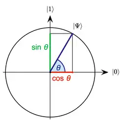
The vector representation of a single qubit is:
- ,

Here, and are the complex probability amplitudes of the qubit. These values determine the probability of measuring a 0 or a 1, when measuring the state of the qubit. See measurement below for details.


The value zero is represented by the ket , and the value one is represented by the ket .


The tensor product (or kronecker product) is used to combine quantum states. The combined state of two qubits is the tensor product of the two qubits. The tensor product is denoted by the symbol .

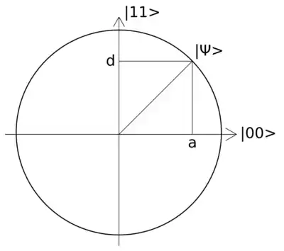
The vector representation of two qubits is:
- ,

The action of the gate on a specific quantum state is found by multiplying the vector which represents the state, by the matrix representing the gate. The result is a new quantum state


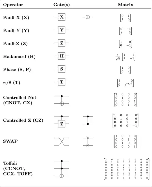
Notable examples
Hadamard (H) gate
The Hadamard gate (French: [adamaʁ]) acts on a single qubit. It maps the basis state to and to , which means that a measurement will have equal probabilities to result in 1 or 0 (i.e. creates a superposition). It represents a rotation of about the axis at the Bloch sphere. Equivalently, it is the combination of two rotations, about the Z-axis, then by about the Y-axis: . It is represented by the Hadamard matrix:


- .

Since where I is the identity matrix, H is a unitary matrix (like all other quantum logical gates).

Pauli-X gate
The Pauli-X gate acts on a single qubit. It is the quantum equivalent of the NOT gate for classical computers (with respect to the standard basis , , which distinguishes the Z-direction; in the sense that a measurement of the eigenvalue +1 corresponds to classical 1/true and -1 to 0/false). It equates to a rotation around the X-axis of the Bloch sphere by radians. It maps to and to . Due to this nature, it is sometimes called bit-flip. It is represented by the Pauli X matrix:
- .

Pauli-Y gate
The Pauli-Y gate acts on a single qubit. It equates to a rotation around the Y-axis of the Bloch sphere by radians. It maps to and to . It is represented by the Pauli Y matrix:


- .

Pauli-Z () gate

The Pauli-Z gate acts on a single qubit. It equates to a rotation around the Z-axis of the Bloch sphere by radians. Thus, it is a special case of a phase shift gate (which are described in a next subsection) with . It leaves the basis state unchanged and maps to . Due to this nature, it is sometimes called phase-flip. It is represented by the Pauli Z matrix:


- .

The Pauli matrices are involutory
The square of a Pauli matrix is the identity matrix.

Square root of NOT gate (√NOT)

The square root of NOT gate (or square root of Pauli-X, ) acts on a single qubit. It maps the basis state to and to .


- .
- .


Phase shift () gates

This is a family of single-qubit gates that map the basis states and . The probability of measuring a or is unchanged after applying this gate, however it modifies the phase of the quantum state. This is equivalent to tracing a horizontal circle (a line of latitude) on the Bloch sphere by radians.


where is the phase shift. Some common examples are the T gate where , the phase gate (written S, though S is sometimes used for SWAP gates) where and the Pauli-Z gate where .


The phase shift gates are related to each other as follows:


Arbitrary single-qubit phase shift gates are natively available for transmon quantum processors through timing of microwave control pulses.[1]
Controlled phase shift
The 2-qubit controlled phase shift gate (sometimes called CPHASE) is:

With respect to the computational basis, it shifts the phase with only if it acts on the state .


Swap (SWAP) gate

The swap gate swaps two qubits. With respect to the basis , , , , it is represented by the matrix:


- .

Square root of Swap gate (√SWAP)

The √SWAP gate performs half-way of a two-qubit swap. It is universal such that any many-qubit gate can be constructed from only √SWAP and single qubit gates. The √SWAP gate is not, however maximally entangling; more than one application of it is required to produce a Bell state from product states. With respect to the basis , , , , it is represented by the matrix:
- .

Controlled (CX CY CZ) gates

Controlled gates act on 2 or more qubits, where one or more qubits act as a control for some operation. For example, the controlled NOT gate (or CNOT or CX) acts on 2 qubits, and performs the NOT operation on the second qubit only when the first qubit is , and otherwise leaves it unchanged. With respect to the basis , , , , it is represented by the matrix:
- .

The CNOT (or controlled Pauli-X) gate can be described as the gate that maps to .


More generally if U is a gate that operates on single qubits with matrix representation
- ,

then the controlled-U gate is a gate that operates on two qubits in such a way that the first qubit serves as a control. It maps the basis states as follows.


The matrix representing the controlled U is
- .


When U is one of the Pauli matrices, σx, σy, or σz, the respective terms "controlled-X", "controlled-Y", or "controlled-Z" are sometimes used.[2] Sometimes this is shortened to just CX, CY and CZ.
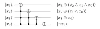
Toffoli (CCNOT) gate

The Toffoli gate, named after Tommaso Toffoli; also called CCNOT gate or Deutsch gate; is a 3-bit gate, which is universal for classical computation but not for quantum computation. The quantum Toffoli gate is the same gate, defined for 3 qubits. If we limit ourselves to only accepting input qubits that are and , then if the first two bits are in the state it applies a Pauli-X (or NOT) on the third bit, else it does nothing. It is an example of a controlled gate. Since it is the quantum analog of a classical gate, it is completely specified by its truth table. The Toffoli gate is universal when combined with the single qubit Hadamard gate.[3]

| Truth table | Matrix form | ||||||||||||||||||||||||||||||||||||||||||||||||||||||
|---|---|---|---|---|---|---|---|---|---|---|---|---|---|---|---|---|---|---|---|---|---|---|---|---|---|---|---|---|---|---|---|---|---|---|---|---|---|---|---|---|---|---|---|---|---|---|---|---|---|---|---|---|---|---|---|
|
| ||||||||||||||||||||||||||||||||||||||||||||||||||||||

It can be also described as the gate which maps to .


Fredkin (CSWAP) gate

The Fredkin gate (also CSWAP or CS gate), named after Edward Fredkin, is a 3-bit gate that performs a controlled swap. It is universal for classical computation. It has the useful property that the numbers of 0s and 1s are conserved throughout, which in the billiard ball model means the same number of balls are output as input.
| Truth table | Matrix form | ||||||||||||||||||||||||||||||||||||||||||||||||||||||||||||
|---|---|---|---|---|---|---|---|---|---|---|---|---|---|---|---|---|---|---|---|---|---|---|---|---|---|---|---|---|---|---|---|---|---|---|---|---|---|---|---|---|---|---|---|---|---|---|---|---|---|---|---|---|---|---|---|---|---|---|---|---|---|
|
| ||||||||||||||||||||||||||||||||||||||||||||||||||||||||||||

Ising (XX) coupling gate
The Ising gate (or XX gate) is a 2-qubit gate that is implemented natively in some trapped-ion quantum computers.[4][5] It is defined as
- ,

Ising (YY) coupling gate
- ,

Ising (ZZ) coupling gate
- ,[6]

Deutsch () gate

The Deutsch (or ) gate, named after physicist David Deutsch is a three-qubit gate. It is defined as

Unfortunately, a working Deutsch gate has remained out of reach, due to lack of a protocol. However, a method was proposed to realize such a Deutsch gate with dipole-dipole interaction in neutral atoms.
Universal quantum gates


Informally, a set of universal quantum gates is any set of gates to which any operation possible on a quantum computer can be reduced, that is, any other unitary operation can be expressed as a finite sequence of gates from the set. Technically, this is impossible with anything less than an uncountable set of gates since the number of possible quantum gates is uncountable, whereas the number of finite sequences from a finite set is countable. To solve this problem, we only require that any quantum operation can be approximated by a sequence of gates from this finite set. Moreover, for unitaries on a constant number of qubits, the Solovay–Kitaev theorem guarantees that this can be done efficiently.
A common universal gate set is the Clifford + T gate set, which is composed of the CNOT, H, S and T gates. (The Clifford set alone is not universal and can be efficiently simulated classically by the Gottesman-Knill theorem.)
A single-gate set of universal quantum gates can also be formulated using the three-qubit Deutsch gate , which performs the transformation[7]

A universal logic gate for reversible classical computing, the Toffoli gate, is reducible to the Deutsch gate, , thus showing that all reversible classical logic operations can be performed on a universal quantum computer.

There also exists a single two-qubit gate sufficient for universality, given it can be applied to any pairs of qubits on a circuit of width .[8]

Another set of universal quantum gates consists of the Ising gate and the phase-shift gate. These are the set of gates natively available in some trapped-ion quantum computers.[5]
Circuit composition
Serially wired gates
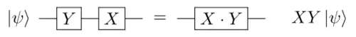
Assume that we have two gates A and B, that both act on qubits. When B is put after A (a series circuit), then the effect of the two gates can be described as a single gate C.

Where is matrix multiplication. The resulting gate C will have the same dimensions as A and B. The order in which the gates would appear in a circuit diagram is reversed when multiplying them together.[9][10]

For example, putting the Pauli X gate after the Pauli Y gate, both of which act on a single qubit, can be described as a single combined gate C:

The product symbol () is often omitted.
Exponents of quantum gates
All real exponents of unitary matrices are also unitary matrices, and all quantum gates are unitary matrices.
Positive integer exponents are equivalent to sequences of serially wired gates (e.g. ), and the real exponents is a generalization of the series circuit. For example, and are both valid quantum gates.


for any unitary matrix . The identity matrix () acts like a NOP and can be represented as bare wire in quantum circuits, or not shown at all.


All gates are unitary matrices, so that and , where is the conjugate transpose. This means that negative exponents of gates are unitary inverses of their positively exponentiated counterparts: . For example, some negative exponents of the phase shift gates are and .


Parallel gates
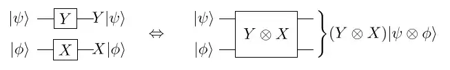


The tensor product (or kronecker product) of two quantum gates is the gate that is equal to the two gates in parallel.[11][12]
If we, as in the picture, combine the Pauli-Y gate with the Pauli-X gate in parallel, then this can be written as:

Both the Pauli-X and the Pauli-Y gate act on a single qubit. The resulting gate act on two qubits.

The Hadamard transform
The gate is the Hadamard gate () applied in parallel on 2 qubits. It can be written as:


This "two-qubit parallel Hadamard gate" will when applied to, for example, the two-qubit zero-vector (), create a quantum state that have equal probability of being observed in any of its four possible outcomes; 00, 01, 10 and 11. We can write this operation as:

Here the amplitude for each measurable state is . The probability to observe any state is the square of the absolute value of the measurable states amplitude, which in the above example means that there is one in four that we observe any one of the individual four cases. See measurement for details.

performs the Hadamard transform on two qubits. Similarly the gate performs a Hadamard transform on a register of qubits.


When applied to a register of qubits all initialized to , the Hadamard transform puts the quantum register into a superposition with equal probability of being measured in any of its possible states:

This state is a uniform superposition and it is generated as the first step in some search algorithms, for example in amplitude amplification and phase estimation.
Measuring this state results in a random number between and . How random the number is depends on the fidelity of the logic gates. If not measured, it is a quantum state with equal probability amplitude for each of its possible states.


The Hadamard transform acts on a register with qubits such that as follows:


Application on entangled states
If two or more qubits are viewed as a single quantum state, this combined state is equal to the tensor product of the constituent qubits. Any state that can be written as a tensor product from the constituent subsystems are called separable states. On the other hand, an entangled state is any state that cannot be tensor-factorized, or in other words: An entangled state can not be written as a tensor product of its constituent qubits states. Special care must be taken when applying gates to constituent qubits that make up entangled states.
If we have a set of N qubits that are entangled and wish to apply a quantum gate on M < N qubits in the set, we will have to extend the gate to take N qubits. This can be done by combining the gate with an identity matrix such that their tensor product becomes a gate that act on N qubits. The identity matrix () is a representation of the gate that maps every state to itself (i.e., does nothing at all). In a circuit diagram the identity gate or matrix will often appear as just a bare wire.


For example, the Hadamard gate () acts on a single qubit, but if we for example feed it the first of the two qubits that constitute the entangled Bell state , we cannot write that operation easily. We need to extend the Hadamard gate with the identity gate so that we can act on quantum states that span two qubits:


The gate can now be applied to any two-qubit state, entangled or otherwise. The gate will leave the second qubit untouched and apply the Hadamard transform to the first qubit. If applied to the Bell state in our example, we may write that as:


The time complexity for multiplying two -matrices is at least ,[13] if using a classical machine. Because the size of a gate that operates on qubits is it means that the time for simulating a step in a quantum circuit (by means of multiplying the gates) that operates on generic entangled states is . For this reason it is believed to be intractable to simulate large entangled quantum systems using classical computers. The Clifford gates is an example of a set of gates that however can be efficiently simulated on classical computers.


Unitary inversion of gates
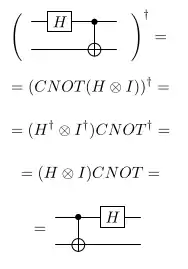

Because all quantum logical gates are reversible, any composition of multiple gates is also reversible. All products and tensor products of unitary matrices are also unitary matrices. This means that it is possible to construct an inverse of all algorithms and functions, as long as they contain only gates.
Initialization, measurement, I/O and spontaneous decoherence are side effects in quantum computers. Gates however are purely functional and bijective.
If a function is a product of gates (), the unitary inverse of the function, , can be constructed:


Because we have, after recursive application on itself


Similarly if the function consists of two gates and in parallel, then and


The dagger () denotes the complex conjugate of the transpose. It is also called the Hermitian adjoint.
Gates that are their own unitary inverses are called Hermitian or self-adjoint operators. Some elementary gates such as the Hadamard (H) and the Pauli gates (I, X, Y, Z) are Hermitian operators, while others like the phase shift (S, T, CPHASE) and the Ising (XX, YY, ZZ) gates generally are not. Gates that are not Hermitian are sometimes called skew-Hermitian, or adjoint operators.
Since is a unitary matrix, and


For example, an algorithm for addition can be used for subtraction, if it is being "run in reverse", as its unitary inverse. The inverse quantum fourier transform is the unitary inverse. Unitary inverses can also be used for uncomputation. Programming languages for quantum computers, such as Microsoft's Q#[14] and Bernhard Ömer's QCL, contain function inversion as programming concepts.
Measurement
Measurement (sometimes called observation) is irreversible and therefore not a quantum gate, because it assigns the observed quantum state to a single value. Measurement takes a quantum state and projects it to one of the basis vectors, with a likelihood equal to the square of the vector's depth (the norm is the modulus squared) along that basis vector.[15][16][17][18] This known as the Born rule and is a stochastic non-reversible operation as it probabilistically sets the quantum state equal to the basis vector that represents the measured state (the state "collapses" to a definite single value). Why and how, or even if[19][20] the quantum state collapses at measurement, is called the measurement problem.
The probability of measuring a value with probability amplitude φ is , where is the modulus.


Measuring a single qubit, whose quantum state is represented by the vector , will result in with probability , and in with probability .


For example, measuring a qubit with the quantum state will yield with equal probability either or .


Note: is the probability of measuring and is the probability of measuring .
A quantum state that spans n qubits can be written as a vector in complex dimensions: . This is because the tensor product of n qubits is a vector in dimensions. This way, a register of n qubits can be measured to distinct states, similar to how a register of n classical bits can hold distinct states. Unlike with the bits of classical computers, quantum states can have non-zero probability amplitudes in multiple measurable values simultaneously. This is called superposition.


The sum of all probabilities for all outcomes must always be equal to 1. Another way to say this is that the Pythagorean theorem generalized to has that all quantum states with n qubits must satisfy , where is the probability amplitude for measurable state . A geometric interpretation of this is that the possible value-space of a quantum state with n qubits is the surface of a unit sphere in and that the unitary transforms (i.e. quantum logic gates) applied to it are rotations on the sphere. Measurement is then a probabilistic projection, or the shadow, of the points at the surface of this complex sphere onto the basis vectors that span the space (and labels the outcomes).


In many cases the space is represented as a Hilbert space rather than some specific -dimensional complex space. The number of dimensions (defined by the basis vectors, and thus also the possible outcomes from measurement) is then often implied by the operands, for example as the required state space for solving a problem. In Grover's algorithm, Lov named this basis vector set "the database".

The selection of basis vectors against to measure a quantum state will influence the outcome of the measurement.[21] See Von Neumann entropy for details. In this article, we always use the computational basis, which means that we have labeled the basis vectors of an n-qubit register , or use the binary representation .


In the quantum computing domain, it is generally assumed that the basis vectors constitute an orthonormal basis.
An example of usage of an alternative measurement basis is in the BB84 cipher.
The effect of measurement on entangled states
If two quantum states (i.e. qubits, or registers) are entangled (meaning that their combined state cannot be expressed as a tensor product), measurement of one register affects or reveals the state of the other register by partially or entirely collapsing its state too. This effect can be used for computation, and is used in many algorithms.
The Hadamard-CNOT combination acts on the zero-state as follows:


This resulting state is the Bell state . It cannot be described as a tensor product of two qubits. There is no solution for


because for example w needs to be both non-zero and zero in the case of xw and yw.
The quantum state spans the two qubits. This is called entanglement. Measuring one of the two qubits that make up this Bell state will result in that the other qubit logically must have the same value, both must be the same: Either it will be found in the state , or in the state . If we measure one of the qubits to be for example , then the other qubit must also be , because their combined state became . Measurement of one of the qubits collapses the entire quantum state, that span the two qubits.
The GHZ state is a similar entangled quantum state that spans three or more qubits.
This type of value-assignment occurs instantaneously over any distance and this has as of 2018 been experimentally verified by QUESS for distances of up to 1200 kilometers.[22][23][24] That the phenomena appears to happen instantaneously as opposed to the time it would take to traverse the distance separating the qubits at the speed of light is called the EPR paradox, and it is an open question in physics how to resolve this. Originally it was solved by giving up the assumption of local realism, but other interpretations have also emerged. For more information see the Bell test experiments. The no-communication theorem proves that this phenomena cannot be used for faster-than-light communication of classical information.
Measurement on registers with pairwise entangled qubits
Take a register A with n qubits all initialized to , and feed it through a parallel Hadamard gate . Register A will then enter the state that have equal probability of when measured to be in any of its possible states; to . Take a second register B, also with n qubits initialized to and pairwise CNOT its qubits with the qubits in register A, such that for each p the qubits and forms the state


If we now measure the qubits in register A, then register B will be found to contain the same value as A. If we however instead apply a quantum logic gate F on A and then measure, then , where is the unitary inverse of F.

Because of how unitary inverses of gates act, . For example, say , then .


The equality will hold no matter in which order measurement is performed (on the registers A or B), assuming that F has run to completion. Measurement can even be randomly and concurrently interleaved qubit by qubit, since the measurements assignment of one qubit will limit the possible value-space from the other entangled qubits.
Even though the equalities holds, the probabilities for measuring the possible outcomes may change as a result of applying F, as may be the intent in a quantum search algorithm.
This effect of value-sharing via entanglement is used in Shor's algorithm, phase estimation and in quantum counting. Using the Fourier transform to amplify the probability amplitudes of the solution states for some problem is a generic method known as "Fourier fishing".
Logic function synthesis
Unitary transformations that are not in the set of gates natively available at the quantum computer (the primitive gates) can be synthesised, or approximated, by combining the available primitive gates in a circuit. One way to do this is to factorize the matrix that encodes the unitary transformation into a product of tensor products (i.e. series and parallel combinations) of the available primitive gates. The group U(2q) is the symmetry group for the gates that act on qubits. The Solovay–Kitaev theorem shows that given a sufficient set of primitive gates, there exist an efficient approximate for any gate. Factorization is then the problem of finding a path in U(2q) from the generating set of primitive gates. For large number of qubits this direct approach to circuit synthesis is intractable for classical computers.[25]
Unitary transformations (functions) that only consist of gates can themselves be fully described as matrices, just like the primitive gates. If a function is a unitary transformation that map qubits from to , then the matrix that represents this transformation have the size . For example, a function that act on a "qubyte" (a register of 8 qubits) would be described as a matrix with elements.


Because the gates unitary nature, all functions must be reversible and always be bijective mappings of input to output. There must always exist a function such that . Functions that are not invertible can be made invertible by adding ancilla qubits to the input or the output, or both. After the function has run to completion, the ancilla qubits can then either be uncomputed or left untouched. Measuring or otherwise collapsing the quantum state of an ancilla qubit (e.g. by re-initializing the value of it, or by its spontaneous decoherence) that have not been uncomputed may result in errors,[26][27] as their state may be entangled with the qubits that are still being used in computations.


Logically irreversible operations, for example addition modulo of two -qubit registers a and b, , can be made logically reversible by adding information to the output, so that the input can be computed from the output (i.e. there exist a function ). In our example, this can be done by passing on one of the input registers to the output: . The output can then be used to compute the input (i.e. given the output and , we can easily find the input; is given and ) and the function is made bijective.


All boolean algebraic expressions can be encoded as unitary transforms (quantum logic gates), for example by using combinations of the Pauli-X, CNOT and Toffoli gates. These gates are functionally complete in the boolean logic domain.
There are many unitary transforms available in the libraries of Q#, QCL, Qiskit, and other quantum programming languages. It also appears in the literature.[28][29]
For example, , where is the number of qubits that constitutes , is implemented as the following in QCL:[30][31]


cond qufunct inc(qureg x) { // increment register
  int i;
  for i = #x-1 to 0 step -1 {
    CNot(x[i], x[0::i]);     // apply controlled-not from
  }                          // MSB to LSB
}
In QCL, decrement is done by "undoing" increment. The undo operator ! is used to instead run the unitary inverse of the function. !inc(x) is the inverse of inc(x) and instead performs the operation .

Here a classic computer generates the gate composition for the quantum computer. The quantum computer acts as a coprocessor that receives instructions from the classical computer about which primitive gates to apply to which qubits.[32] Measurement of quantum registers results in binary values that the classical computer can use in its computations. Quantum algorithms often contain both a classical and a quantum part. Unmeasured I/O (sending qubits to remote computers without collapsing their quantum states) can be used to create networks of quantum computers. Entanglement swapping can then be used to realize distributed algorithms with quantum computers that are not directly connected. Examples of distributed algorithms that only require the use of a handful of quantum logic gates is superdense coding, the Quantum Byzantine agreement and the BB84 cipherkey exchange protocol.
History
The current notation for quantum gates was developed by Barenco et al.,[33] building on notation introduced by Feynman.[34]
See also
- Adiabatic quantum computation
- Cellular automaton and Quantum cellular automaton
- Classical computing and Quantum computing
- Classic logic gate
- Cloud-based quantum computing
- Computational complexity theory and BQP
- Counterfactual definiteness and Counterfactual computation
- DiVincenzo's criteria
- Landauer's principle and reversible computation, decoherence
- Magic state distillation
- Information theory, quantum information and Von Neumann entropy
- Pauli effect and Synchronicity
- Pauli matrices
- Quantum algorithms
- Quantum circuit
- Quantum error correction
- Quantum finite automata
- Quantum memory
- Quantum network and Quantum channel
- Quantum state
- U(2q) and SU(2q) where is the number of qubits the gates act on
- Unitary transformations in quantum mechanics
- Zeno effect
References
- Dibyendu Chatterjee, Arijit Roy (2015). "A transmon-based quantum half-adder scheme". Progress of Theoretical and Experimental Physics. 2015 (9): 7–8. Bibcode:2015PTEP.2015i3A02C. doi:10.1093/ptep/ptv122.
- Nielsen, Michael A.; Chuang, Isaac (2000). Quantum Computation and Quantum Information. Cambridge: Cambridge University Press. ISBN 0521632358. OCLC 43641333.
- Aharonov, Dorit (2003-01-09). "A Simple Proof that Toffoli and Hadamard are Quantum Universal". arXiv:quant-ph/0301040.
- "Monroe Conference" (PDF). online.kitp.ucsb.edu.
- "Demonstration of a small programmable quantum computer with atomic qubits" (PDF). Retrieved 2019-02-10.
- Jones, Jonathan A. (2003). "Robust Ising gates for practical quantum computation". Physical Review A. 67 (1): 012317. arXiv:quant-ph/0209049. Bibcode:2003PhRvA..67a2317J. doi:10.1103/PhysRevA.67.012317. S2CID 119421647.
- Deutsch, David (September 8, 1989), "Quantum computational networks", Proc. R. Soc. Lond. A, 425 (1989): 73–90, Bibcode:1989RSPSA.425...73D, doi:10.1098/rspa.1989.0099, S2CID 123073680
- Bausch, Johannes; Piddock, Stephen (2017), "The Complexity of Translationally-Invariant Low-Dimensional Spin Lattices in 3D", Journal of Mathematical Physics, 58 (11): 111901, arXiv:1702.08830, Bibcode:2017JMP....58k1901B, doi:10.1063/1.5011338, S2CID 8502985
- Yanofsky, Noson S.; Mannucci, Mirco (2013). Quantum computing for computer scientists. Cambridge University Press. pp. 147–169. ISBN 978-0-521-87996-5.
- Nielsen, Michael A.; Chuang, Isaac (2000). Quantum Computation and Quantum Information. Cambridge: Cambridge University Press. pp. 62–63. ISBN 0521632358. OCLC 43641333.
- Yanofsky, Noson S.; Mannucci, Mirco (2013). Quantum computing for computer scientists. Cambridge University Press. p. 148. ISBN 978-0-521-87996-5.
- Nielsen, Michael A.; Chuang, Isaac (2000). Quantum Computation and Quantum Information. Cambridge: Cambridge University Press. pp. 71–75. ISBN 0521632358. OCLC 43641333.
- Raz, Ran (2002). "On the complexity of matrix product". Proceedings of the Thirty-fourth Annual ACM Symposium on Theory of Computing: 144. doi:10.1145/509907.509932. ISBN 1581134959. S2CID 9582328.
- Defining adjoined operators in Microsof Q#
- Griffiths, D.J. (1987). Introduction to Elementary Particles. John Wiley & Sons. pp. 115–121, 126. ISBN 0-471-60386-4.
- Colin P. Williams (2011). Explorations in Quantum Computing. Springer. pp. 15–17. ISBN 978-1-84628-887-6.
- David Albert (1994). Quantum mechanics and experience. Harvard University Press. p. 35. ISBN 0-674-74113-7.
- Sean M. Carroll (2019). Spacetime and geometry: An introduction to general relativity. Cambridge University Press. pp. 376–394. ISBN 978-1-108-48839-6.
- David Wallace (2012). The emergent multiverse: Quantum theory according to the Everett Interpretation. Oxford University Press. ISBN 9780199546961.
- Sean M. Carroll (2019). Something deeply hidden: Quantum worlds and the emergence of spacetime. Penguin Random House. ISBN 9781524743017.
- Q# Online manual: Measurement
- Juan Yin, Yuan Cao, Yu-Huai Li, et.c. (2017). "Satellite-based entanglement distribution over 1200 kilometers". Quantum Optics. 356: 1140–1144. arXiv:1707.01339.CS1 maint: uses authors parameter (link)
- Billings, Lee. "China Shatters "Spooky Action at a Distance" Record, Preps for Quantum Internet". Scientific American.
- Popkin, Gabriel (15 June 2017). "China's quantum satellite achieves 'spooky action' at record distance". Science - AAAS.
- Matteo, Olivia Di (2016). "Parallelizing quantum circuit synthesis". Quantum Science and Technology. 1 (1): 015003. arXiv:1606.07413. Bibcode:2016QS&T....1a5003D. doi:10.1088/2058-9565/1/1/015003. S2CID 62819073.
- Aaronson, Scott (2002). "Quantum Lower Bound for Recursive Fourier Sampling". Quantum Information and Computation. 3 (2): 165–174. arXiv:quant-ph/0209060. Bibcode:2002quant.ph..9060A.
- Q# online manual: Quantum Memory Management
- Ryo, Asaka; Kazumitsu, Sakai; Ryoko, Yahagi (2020). "Quantum circuit for the fast Fourier transform". Quantum Information Processing. 19 (277): 277. arXiv:1911.03055. Bibcode:2020QuIP...19..277A. doi:10.1007/s11128-020-02776-5. S2CID 207847474.
- Montaser, Rasha (2019). "New Design of Reversible Full Adder/Subtractor using R gate". International Journal of Theoretical Physics. 58 (1): 167–183. arXiv:1708.00306. Bibcode:2019IJTP...58..167M. doi:10.1007/s10773-018-3921-1. S2CID 24590164.
- QCL 0.6.4 source code, the file "lib/examples.qcl"
- Quantum Programming in QCL (PDF)
- S. J. Pauka, K. Das, R. Kalra, A. Moini, Y. Yang, M. Trainer, A. Bousquet, C. Cantaloube, N. Dick, G. C. Gardner, M. J. (2021). "A cryogenic CMOS chip for generating control signals for multiple qubits". Nature Electronics (4). arXiv:1912.01299. doi:10.1038/s41928-020-00528-y.CS1 maint: uses authors parameter (link)
- Phys. Rev. A 52 3457–3467 (1995), doi:10.1103/PhysRevA.52.3457; e-print arXiv:quant-ph/9503016
- R. P. Feynman, "Quantum mechanical computers", Optics News, February 1985, 11, p. 11; reprinted in Foundations of Physics 16(6) 507–531.
Sources
- Nielsen, Michael A.; Chuang, Isaac (2000). Quantum Computation and Quantum Information. Cambridge: Cambridge University Press. ISBN 0521632358. OCLC 43641333.
- Yanofsky, Noson S.; Mannucci, Mirco (2013). Quantum computing for computer scientists. Cambridge University Press. ISBN 978-0-521-87996-5.
| General |  | ||||||||
|---|---|---|---|---|---|---|---|---|---|
| Theorems | |||||||||
| Quantum communication | |||||||||
| Quantum algorithms | |||||||||
| Quantum complexity theory | |||||||||
| Quantum computing models | |||||||||
| Quantum error correction | |||||||||
| Physical implementations |
| ||||||||
| Software |
| ||||||||
| |||||||||
