Moving average
In statistics, a moving average (rolling average or running average) is a calculation to analyze data points by creating a series of averages of different subsets of the full data set. It is also called a moving mean (MM)[1] or rolling mean and is a type of finite impulse response filter. Variations include: simple, and cumulative, or weighted forms (described below).
Given a series of numbers and a fixed subset size, the first element of the moving average is obtained by taking the average of the initial fixed subset of the number series. Then the subset is modified by "shifting forward"; that is, excluding the first number of the series and including the next value in the subset.
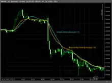
A moving average is commonly used with time series data to smooth out short-term fluctuations and highlight longer-term trends or cycles. The threshold between short-term and long-term depends on the application, and the parameters of the moving average will be set accordingly. For example, it is often used in technical analysis of financial data, like stock prices, returns or trading volumes. It is also used in economics to examine gross domestic product, employment or other macroeconomic time series. Mathematically, a moving average is a type of convolution and so it can be viewed as an example of a low-pass filter used in signal processing. When used with non-time series data, a moving average filters higher frequency components without any specific connection to time, although typically some kind of ordering is implied. Viewed simplistically it can be regarded as smoothing the data.
Simple moving average (boxcar filter)
In financial applications a simple moving average (SMA) is the unweighted mean of the previous data-points. However, in science and engineering, the mean is normally taken from an equal number of data on either side of a central value. This ensures that variations in the mean are aligned with the variations in the data rather than being shifted in time. An example of a simple equally weighted running mean for a -day sample of the closing price is the mean of the previous days' closing prices. Let those prices be . Let the mean over the first data-points be . Thus, the mean over all the data-points is calculated as:


This means that the moving average filter can be computed quite cheaply on real time data with a FIFO / circular buffer.
When calculating successive values, a new value comes into the sum, and the oldest value drops out. This means that a full summation each time is unnecessary. Thus, the new mean can be calculated as:

The period selected depends on the type of movement of interest, such as short, intermediate, or long-term. In financial terms, moving-average levels can be interpreted as support in a falling market or resistance in a rising market.
If the data used are not centered around the mean, a simple moving average lags behind the latest datum point by half the sample width. An SMA can also be disproportionately influenced by old datum points dropping out or new data coming in. One characteristic of the SMA is that if the data have a periodic fluctuation, then applying an SMA of that period will eliminate that variation (the average always containing one complete cycle). But a perfectly regular cycle is rarely encountered.[2]
For a number of applications, it is advantageous to avoid the shifting induced by using only "past" data. Hence a central moving average can be computed, using data equally spaced on either side of the point in the series where the mean is calculated.[3] This requires using an odd number of datum points in the sample window.
A major drawback of the SMA is that it lets through a significant amount of the signal shorter than the window length. Worse, it actually inverts it. This can lead to unexpected artifacts, such as peaks in the smoothed result appearing where there were troughs in the data. It also leads to the result being less smooth than expected since some of the higher frequencies are not properly removed.
Cumulative moving average
In a cumulative moving average (CMA), the data arrive in an ordered datum stream, and the user would like to get the average of all of the data up until the current datum point. For example, an investor may want the average price of all of the stock transactions for a particular stock up until the current time. As each new transaction occurs, the average price at the time of the transaction can be calculated for all of the transactions up to that point using the cumulative average, typically an equally weighted average of the sequence of n values up to the current time:


The brute-force method to calculate this would be to store all of the data and calculate the sum and divide by the number of datum points every time a new datum point arrived. However, it is possible to simply update cumulative average as a new value, becomes available, using the formula


Thus the current cumulative average for a new datum point is equal to the previous cumulative average, times n, plus the latest datum point, all divided by the number of points received so far, n+1. When all of the datum points arrive (n = N), then the cumulative average will equal the final average. It is also possible to store a running total of the datum point as well as the number of points and dividing the total by the number of datum points to get the CMA each time a new datum point arrives.
The derivation of the cumulative average formula is straightforward. Using

and similarly for n + 1, it is seen that

Solving this equation for results in


Weighted moving average
A weighted average is an average that has multiplying factors to give different weights to data at different positions in the sample window. Mathematically, the weighted moving average is the convolution of the datum points with a fixed weighting function. One application is removing pixelisation from a digital graphical image.
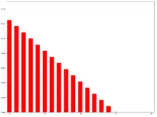
In technical analysis of financial data, a weighted moving average (WMA) has the specific meaning of weights that decrease in arithmetical progression.[4] In an n-day WMA the latest day has weight n, the second latest n − 1, etc., down to one.

The denominator is a triangle number equal to In the more general case the denominator will always be the sum of the individual weights.

When calculating the WMA across successive values, the difference between the numerators of WMAM+1 and WMAM is npM+1 − pM − ⋅⋅⋅ − pM−n+1. If we denote the sum pM + ⋅⋅⋅ + pM−n+1 by TotalM, then

The graph at the right shows how the weights decrease, from highest weight for the most recent datum points, down to zero. It can be compared to the weights in the exponential moving average which follows.
Exponential moving average
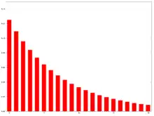
An exponential moving average (EMA), also known as an exponentially weighted moving average (EWMA),[5] is a first-order infinite impulse response filter that applies weighting factors which decrease exponentially. The weighting for each older datum decreases exponentially, never reaching zero. The graph at right shows an example of the weight decrease.
The EMA for a series Y may be calculated recursively:

Where:
- The coefficient α represents the degree of weighting decrease, a constant smoothing factor between 0 and 1. A higher α discounts older observations faster.
- Yt is the value at a time period t.
- St is the value of the EMA at any time period t.
S1 may be initialized in a number of different ways, most commonly by setting S1 to Y1 as shown above, though other techniques exist, such as setting S1 to an average of the first 4 or 5 observations. The importance of the S1 initialisations effect on the resultant moving average depends on α; smaller α values make the choice of S1 relatively more important than larger α values, since a higher α discounts older observations faster.
Whatever is done for S1 it assumes something about values prior to the available data and is necessarily in error. In view of this, the early results should be regarded as unreliable until the iterations have had time to converge. This is sometimes called a 'spin-up' interval. One way to assess when it can be regarded as reliable is to consider the required accuracy of the result. For example, if 3% accuracy is required, initialising with Y1 and taking data after five time constants (defined above) will ensure that the calculation has converged to within 3% (only <3% of Y1 will remain in the result). Sometimes with very small alpha, this can mean little of the result is useful. This is analogous to the problem of using a convolution filter (such as a weighted average) with a very long window.
This formulation is according to Hunter (1986).[6] By repeated application of this formula for different times, we can eventually write St as a weighted sum of the datum points Yt, as:

for any suitable k ∈ {0, 1, 2, ...} The weight of the general datum point is .


This formula can also be expressed in technical analysis terms as follows, showing how the EMA steps towards the latest datum point, but only by a proportion of the difference (each time):

Expanding out each time results in the following power series, showing how the weighting factor on each datum point p1, p2, etc., decreases exponentially:


where
- is
- is
- and so on


since .

It can also be calculated recursively without introducing the error when initializing the first estimate (n starts from 1):
- Assume


This is an infinite sum with decreasing terms.
Approximating the EMA with a limited number of terms
The question of how far back to go for an initial value depends, in the worst case, on the data. Large price values in old data will affect the total even if their weighting is very small. If prices have small variations then just the weighting can be considered. The power formula above gives a starting value for a particular day, after which the successive days formula shown first can be applied. The weight omitted by stopping after k terms is

which is

i.e. a fraction

out of the total weight.
For example, to have 99.9% of the weight, set above ratio equal to 0.1% and solve for k:

to determine how many terms should be used. Since as , we know approaches as N increases .[8] This gives:


When is related to N as , this simplifies to approximately[9]


for this example (99.9% weight).
Relationship between SMA and EMA
Note that there is no "accepted" value that should be chosen for , although there are some recommended values based on the application. A commonly used value for is . This is because the weights of an SMA and EMA have the same "center of mass" when .


The weights of an -day SMA have a "center of mass" on the day, where


(or , if we use zero-based indexing)

For the remainder of this proof we will use one-based indexing.
Now meanwhile, the weights of an EMA have center of mass

That is,

We also know the Maclaurin Series

Taking derivatives of both sides with respect to gives:


or

Substituting , we get


or

So the value of that sets is, in fact:


or

And so is the value of that creates an EMA whose weights have the same center of gravity as would the equivalent N-day SMA

This is also why sometimes an EMA is referred to as an N-day EMA. Despite the name suggesting there are N periods, the terminology only specifies the α factor. N is not a stopping point for the calculation in the way it is in an SMA or WMA. For sufficiently large N, the first N datum points in an EMA represent about 86% of the total weight in the calculation when :
The sum of the weights of all the terms (i.e., infinite number of terms) in an exponential moving average is 1. The sum of the weights of terms is . Both of these sums can be derived by using the formula for the sum of a geometric series. The weight omitted after terms is given by subtracting this from 1, and you get (this is essentially the formula given previously for the weight omitted).


We now substitute the commonly used value for in the formula for the weight of terms. If you make this substitution, and you make use of[10] , then you get


- i.e. simplified,[12] tends to .


the 0.8647 approximation. Intuitively, what this is telling us is that the weight after terms of an ``-period" exponential moving average converges to 0.8647.
The designation of is not a requirement. (For example, a similar proof could be used to just as easily determine that the EMA with a half-life of N-days is or that the EMA with the same median as an N-day SMA is ). In fact, 2/(N+1) is merely a common convention to form an intuitive understanding of the relationship between EMAs and SMAs, for industries where both are commonly used together on the same datasets. In reality, an EMA with any value of can be used, and can be named either by stating the value of , or with the more familiar N-day EMA terminology letting .


Exponentially weighted moving variance and standard deviation
In addition to the mean, we may also be interested in the variance and in the standard deviation to evaluate the statistical significance of a deviation from the mean.
EWMVar can be computed easily along with the moving average. The starting values are and , and we then compute the subsequent values using:[13]


From this, the exponentially weighted moving standard deviation can be computed as . We can then use the standard score to normalize data with respect to the moving average and variance. This algorithm is based on Welford's algorithm for computing the variance.

Modified moving average
A modified moving average (MMA), running moving average (RMA), or smoothed moving average (SMMA) is defined as:

In short, this is an exponential moving average, with .

Application to measuring computer performance
Some computer performance metrics, e.g. the average process queue length, or the average CPU utilization, use a form of exponential moving average.

Here α is defined as a function of time between two readings. An example of a coefficient giving bigger weight to the current reading, and smaller weight to the older readings is

where exp() is the exponential function, time for readings tn is expressed in seconds, and W is the period of time in minutes over which the reading is said to be averaged (the mean lifetime of each reading in the average). Given the above definition of α, the moving average can be expressed as

For example, a 15-minute average L of a process queue length Q, measured every 5 seconds (time difference is 5 seconds), is computed as

Other weightings
Other weighting systems are used occasionally – for example, in share trading a volume weighting will weight each time period in proportion to its trading volume.
A further weighting, used by actuaries, is Spencer's 15-Point Moving Average[14] (a central moving average). Its symmetric weight coefficients are [−3, −6, −5, 3, 21, 46, 67, 74, 67, 46, 21, 3, −5, −6, −3], which factors as [1, 1, 1, 1]*[1, 1, 1, 1]*[1, 1, 1, 1, 1]*[−3, 3, 4, 3, −3]/320 and leaves samples of any cubic polynomial unchanged.[15]
Outside the world of finance, weighted running means have many forms and applications. Each weighting function or "kernel" has its own characteristics. In engineering and science the frequency and phase response of the filter is often of primary importance in understanding the desired and undesired distortions that a particular filter will apply to the data.
A mean does not just "smooth" the data. A mean is a form of low-pass filter. The effects of the particular filter used should be understood in order to make an appropriate choice. On this point, the French version of this article discusses the spectral effects of 3 kinds of means (cumulative, exponential, Gaussian).
Moving median
From a statistical point of view, the moving average, when used to estimate the underlying trend in a time series, is susceptible to rare events such as rapid shocks or other anomalies. A more robust estimate of the trend is the simple moving median over n time points:

where the median is found by, for example, sorting the values inside the brackets and finding the value in the middle. For larger values of n, the median can be efficiently computed by updating an indexable skiplist.[16]
Statistically, the moving average is optimal for recovering the underlying trend of the time series when the fluctuations about the trend are normally distributed. However, the normal distribution does not place high probability on very large deviations from the trend which explains why such deviations will have a disproportionately large effect on the trend estimate. It can be shown that if the fluctuations are instead assumed to be Laplace distributed, then the moving median is statistically optimal.[17] For a given variance, the Laplace distribution places higher probability on rare events than does the normal, which explains why the moving median tolerates shocks better than the moving mean.
When the simple moving median above is central, the smoothing is identical to the median filter which has applications in, for example, image signal processing.
Moving average regression model
In a moving average regression model, a variable of interest is assumed to be a weighted moving average of unobserved independent error terms; the weights in the moving average are parameters to be estimated.
Those two concepts are often confused due to their name, but while they share many similarities, they represent distinct methods and are used in very different contexts.
See also
| Wikimedia Commons has media related to Moving averages. |
Notes and references
- Hydrologic Variability of the Cosumnes River Floodplain (Booth et al., San Francisco Estuary and Watershed Science, Volume 4, Issue 2, 2006)
- Statistical Analysis, Ya-lun Chou, Holt International, 1975, ISBN 0-03-089422-0, section 17.9.
- The derivation and properties of the simple central moving average are given in full at Savitzky–Golay filter.
- "Weighted Moving Averages: The Basics". Investopedia.
- "Archived copy". Archived from the original on 2010-03-29. Retrieved 2010-10-26.CS1 maint: archived copy as title (link)
- NIST/SEMATECH e-Handbook of Statistical Methods: Single Exponential Smoothing at the National Institute of Standards and Technology
- The Maclaurin Series for is
- It means , and the Taylor series of approaches .
- loge(0.001) / 2 = −3.45
- See the following link for a proof.
- The denominator on the left-hand side should be unity, and the numerator will become the right-hand side (geometric series), .
- Because (1 + x/n)n tends to the limit ex for large n.
- Finch, Tony. "Incremental calculation of weighted mean and variance" (PDF). University of Cambridge. Retrieved 19 December 2019.
- Spencer's 15-Point Moving Average — from Wolfram MathWorld
- Rob J Hyndman. "Moving averages". 2009-11-08. Accessed 2020-08-20.
- "Efficient Running Median using an Indexable Skiplist « Python recipes « ActiveState Code".
- G.R. Arce, "Nonlinear Signal Processing: A Statistical Approach", Wiley:New Jersey, USA, 2005.


