Radiation pattern
In the field of antenna design the term radiation pattern (or antenna pattern or far-field pattern) refers to the directional (angular) dependence of the strength of the radio waves from the antenna or other source.[1][2][3]
Particularly in the fields of fiber optics, lasers, and integrated optics, the term radiation pattern may also be used as a synonym for the near-field pattern or Fresnel pattern.[4] This refers to the positional dependence of the electromagnetic field in the near-field, or Fresnel region of the source. The near-field pattern is most commonly defined over a plane placed in front of the source, or over a cylindrical or spherical surface enclosing it.[1][4]
The far-field pattern of an antenna may be determined experimentally at an antenna range, or alternatively, the near-field pattern may be found using a near-field scanner, and the radiation pattern deduced from it by computation.[1] The far-field radiation pattern can also be calculated from the antenna shape by computer programs such as NEC. Other software, like HFSS can also compute the near field.
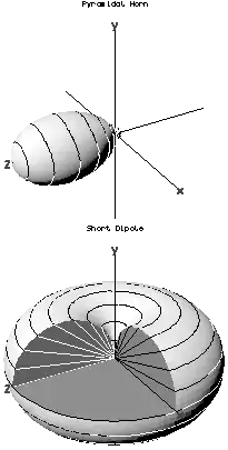
The far field radiation pattern may be represented graphically as a plot of one of a number of related variables, including; the field strength at a constant (large) radius (an amplitude pattern or field pattern), the power per unit solid angle (power pattern) and the directive gain. Very often, only the relative amplitude is plotted, normalized either to the amplitude on the antenna boresight, or to the total radiated power. The plotted quantity may be shown on a linear scale, or in dB. The plot is typically represented as a three-dimensional graph (as at right), or as separate graphs in the vertical plane and horizontal plane. This is often known as a polar diagram.
Reciprocity
It is a fundamental property of antennas that the receiving pattern (sensitivity as a function of direction) of an antenna when used for receiving is identical to the far-field radiation pattern of the antenna when used for transmitting. This is a consequence of the reciprocity theorem of electro-magnetics and is proved below. Therefore, in discussions of radiation patterns the antenna can be viewed as either transmitting or receiving, whichever is more convenient. Note however that this applies only to the passive antenna elements. Active antennas that include amplifiers or other components are no longer reciprocal devices.
Typical patterns
Since electromagnetic radiation is dipole radiation, it is not possible to build an antenna that radiates coherently equally in all directions, although such a hypothetical isotropic antenna is used as a reference to calculate antenna gain.
The simplest antennas, monopole and dipole antennas, consist of one or two straight metal rods along a common axis. These axially symmetric antennas have radiation patterns with a similar symmetry, called omnidirectional patterns; they radiate equal power in all directions perpendicular to the antenna, with the power varying only with the angle to the axis, dropping off to zero on the antenna's axis. This illustrates the general principle that if the shape of an antenna is symmetrical, its radiation pattern will have the same symmetry.
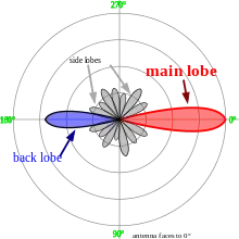
In most antennas, the radiation from the different parts of the antenna interferes at some angles; the radiation pattern of the antenna can be considered an interference pattern. This results in zero radiation at certain angles where the radio waves from the different parts arrive out of phase, and local maxima of radiation at other angles where the radio waves arrive in phase. Therefore, the radiation plot of most antennas shows a pattern of maxima called "lobes" at various angles, separated by "nulls" at which the radiation goes to zero. The larger the antenna is compared to a wavelength, the more lobes there will be.
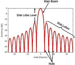
In a directional antenna in which the objective is to emit the radio waves in one particular direction, the antenna is designed to radiate most of its power in the lobe directed in the desired direction. Therefore in the radiation plot this lobe appears larger than the others; it is called the "main lobe". The axis of maximum radiation, passing through the center of the main lobe, is called the "beam axis" or boresight axis". In some antennas, such as split-beam antennas, there may exist more than one major lobe. The other lobes beside the main lobe, representing unwanted radiation in other directions, are called minor lobes. The minor lobes oriented at an angle to the main lobe are called "side lobes". The minor lobe in the opposite direction (180°) from the main lobe is called the "back lobe".
Minor lobes usually represent radiation in undesired directions, so in directional antennas a design goal is usually to reduce the minor lobes. Side lobes are normally the largest of the minor lobes. The level of minor lobes is usually expressed as a ratio of the power density in the lobe in question to that of the major lobe. This ratio is often termed the side lobe ratio or side lobe level. Side lobe levels of −20 dB or greater are usually not desirable in many applications. Attainment of a side lobe level smaller than −30 dB usually requires very careful design and construction. In most radar systems, for example, low side lobe ratios are very important to minimize false target indications through the side lobes.
Proof of reciprocity
| Part of a series on |
| Antennas |
|---|
 |
For a complete proof, see the reciprocity (electromagnetism) article. Here, we present a common simple proof limited to the approximation of two antennas separated by a large distance compared to the size of the antenna, in a homogeneous medium. The first antenna is the test antenna whose patterns are to be investigated; this antenna is free to point in any direction. The second antenna is a reference antenna, which points rigidly at the first antenna.
Each antenna is alternately connected to a transmitter having a particular source impedance, and a receiver having the same input impedance (the impedance may differ between the two antennas).
It is assumed that the two antennas are sufficiently far apart that the properties of the transmitting antenna are not affected by the load placed upon it by the receiving antenna. Consequently, the amount of power transferred from the transmitter to the receiver can be expressed as the product of two independent factors; one depending on the directional properties of the transmitting antenna, and the other depending on the directional properties of the receiving antenna.
For the transmitting antenna, by the definition of gain, , the radiation power density at a distance from the antenna (i.e. the power passing through unit area) is


- .

Here, the angles and indicate a dependence on direction from the antenna, and stands for the power the transmitter would deliver into a matched load. The gain may be broken down into three factors; the antenna gain (the directional redistribution of the power), the radiation efficiency (accounting for ohmic losses in the antenna), and lastly the loss due to mismatch between the antenna and transmitter. Strictly, to include the mismatch, it should be called the realized gain,[4] but this is not common usage.


For the receiving antenna, the power delivered to the receiver is
- .

Here is the power density of the incident radiation, and is the antenna aperture or effective area of the antenna (the area the antenna would need to occupy in order to intercept the observed captured power). The directional arguments are now relative to the receiving antenna, and again is taken to include ohmic and mismatch losses.


Putting these expressions together, the power transferred from transmitter to receiver is
- ,

where and are directionally dependent properties of the transmitting and receiving antennas respectively. For transmission from the reference antenna (2), to the test antenna (1), that is
- ,

and for transmission in the opposite direction
- .

Here, the gain and effective area of antenna 2 are fixed, because the orientation of this antenna is fixed with respect to the first.


Now for a given disposition of the antennas, the reciprocity theorem requires that the power transfer is equally effective in each direction, i.e.
- ,

whence
- .

But the right hand side of this equation is fixed (because the orientation of antenna 2 is fixed), and so
- ,

i.e. the directional dependence of the (receiving) effective aperture and the (transmitting) gain are identical (QED). Furthermore, the constant of proportionality is the same irrespective of the nature of the antenna, and so must be the same for all antennas. Analysis of a particular antenna (such as a Hertzian dipole), shows that this constant is , where is the free-space wavelength. Hence, for any antenna the gain and the effective aperture are related by


- .

Even for a receiving antenna, it is more usual to state the gain than to specify the effective aperture. The power delivered to the receiver is therefore more usually written as

(see link budget). The effective aperture is however of interest for comparison with the actual physical size of the antenna.
Practical consequences
- When determining the pattern of a receiving antenna by computer simulation, it is not necessary to perform a calculation for every possible angle of incidence. Instead, the radiation pattern of the antenna is determined by a single simulation, and the receiving pattern inferred by reciprocity.
- When determining the pattern of an antenna by measurement, the antenna may be either receiving or transmitting, whichever is more convenient.
- For a practical antenna, the side lobe level should be minimum, it is necessary to have the maximum directivity.[5]
See also
References
- Constantine A. Balanis: “Antenna Theory, Analysis and Design”, John Wiley & Sons, Inc., 2nd ed. 1982 ISBN 0-471-59268-4
- David K Cheng: “Field and Wave Electromagnetics”, Addison-Wesley Publishing Company Inc., Edition 2, 1998. ISBN 0-201-52820-7
- Edward C. Jordan & Keith G. Balmain; “Electromagnetic Waves and Radiating Systems” (2nd ed. 1968) Prentice-Hall. ISBN 81-203-0054-8
- Institute of Electrical and Electronics Engineers, “The IEEE standard dictionary of electrical and electronics terms”; 6th ed. New York, N.Y., Institute of Electrical and Electronics Engineers, c1997. IEEE Std 100-1996. ISBN 1-55937-833-6 [ed. Standards Coordinating Committee 10, Terms and Definitions; Jane Radatz, (chair)]
- Singh, Urvinder; Salgotra, Rohit (20 July 2016). "Synthesis of linear antenna array using flower pollination algorithm". Neural Computing and Applications. 29 (2): 435–445. doi:10.1007/s00521-016-2457-7.
![]() This article incorporates public domain material from the General Services Administration document: "Federal Standard 1037C". (in support of MIL-STD-188)
This article incorporates public domain material from the General Services Administration document: "Federal Standard 1037C". (in support of MIL-STD-188)
External links
- Understanding and Using Antenna Radiation Patterns By Joseph H. Reisert
- Explanation of the term “Two-Way beamwidth”
